How to deploy your deep learning side project on a budget

Imagine this scenario: you have successfully trained a nice big neural network model for your side project. The next step is deploying it, making it available for everyone to use and benefit from. However, you quickly realize that deploying your model is easier said than done. Running your model solely on a CPU would be too slow, but upon exploring GPU offerings, you are confronted with a disheartening reality – keeping a GPU running, even for the most basic on-demand g4dn instance on AWS, would cost an exorbitant $400 USD per month, which is probably more than you are willing to pay for hosting your side project. Not to mention, in the beginning when you may only receive a few requests a day, keeping such a powerful GPU instance feels wasteful. You may wonder: what viable alternatives exist? How can you deploy your model affordably without compromising on availability and latency?

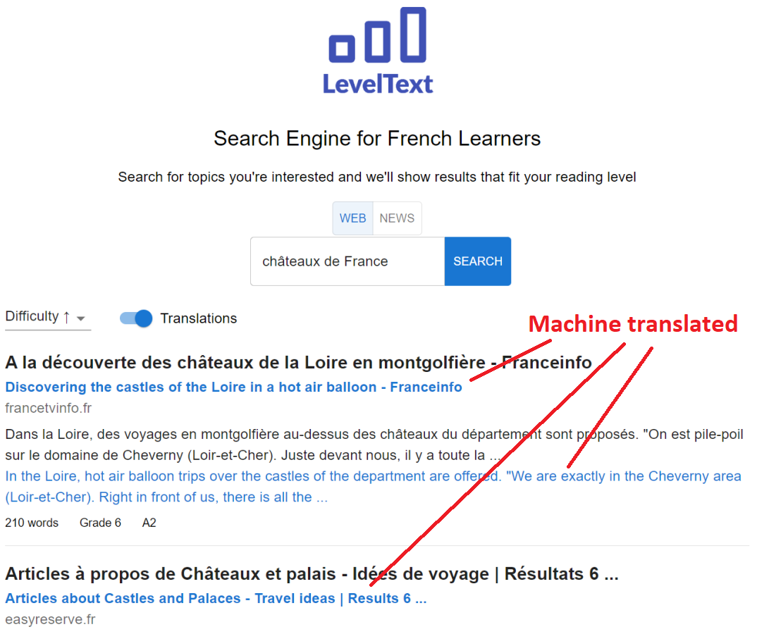
This is exactly the challenge we encountered when deploying our Efficient NLP translation models. To give you some context, Efficient NLP is the translation engine powering LevelText, a language learning app that I developed. In LevelText, users perform searches for articles on the web in a foreign language, and our backend must translate a bunch of web articles in real-time to return the result. So the translation needs to happen fairly quickly or else the user will get impatient and go do something else.

We decided to deploy our model with serverless GPUs. In the serverless computing architecture, instead of managing instances, you define functions that are triggered by specific events, such as an HTTP request. Typically you package up your model and inference code into a Docker container, and push the docker image to a cloud registry like AWS ECR. The beauty of serverless lies in its automated resource provisioning – the platform takes care of allocating and shutting down resources as needed to execute your function. The good news is you only pay for when the function is actually run, so your cost will be as low as a few dollars rather than hundreds of dollars a month if the function is idle most of the time. Also, if your side project suddenly ends up on Hacker News and gains traction, serverless allows you to automatically scale up to meet the demand without additional engineering effort.

When it comes to serverless for deep learning models, several challenges arise. The first is that AWS (as well as other major cloud providers like GCP and Azure) does not currently offer serverless GPUs. AWS provides several serverless options like Lambda and SageMaker Serverless Inference, but they are limited to CPU usage only. This limitation stems from their underlying infrastructure: AWS serverless services including Lambda and Fargate are built on Firecracker, a virtualization engine designed for quickly and securely spinning up serverless containers, but Firecracker has no GPU support.

With serverless computing, the most crucial metric is the time to start up a container, commonly known as cold start time. This rules out alternative options such as spinning up EC2 instances on-demand to handle requests: while EC2 instances offer GPU capabilities, they are not optimized for quick startup times (typically taking around 40 seconds to start up), which is impractical for time-sensitive applications.

Fortunately, there are a number of startups that have emerged to fill this gap and offer serverless GPUs, such as Banana, Runpod, Modal, Replicate, and many more. They are similar but differ on cold start time, availability and pricing of different GPUs, and configuration options. We evaluated several and opted for one of these startups, but the serverless GPU landscape is quickly evolving, and the most suitable option for you may be none of the above by the time you read this.

Also worth noting: before choosing a serverless GPU startup, it’s a good idea to do some benchmarks and see if it’s really not possible to deploy your model on a CPU instance. With multicore processors, instances with large memory, newer CPU instruction sets like AVX-512, often running the model on CPUs may be fast enough. Generally deploying on CPUs will be easier and you will have more options available to choose from on the major cloud providers.

The next step is making your model smaller and/or faster. This can be achieved through several different approaches:

• Quantization: This means reducing the precision of each weight in the model, such as from fp32 to fp16 or int8 or sometimes even smaller. Converting from fp32 to int8 means a 4x reduction in model size. There are several different types of quantization, in particular for int8 quantization there is the issue of determining the scale factor (how to convert values between float values and integers between 0-255): the easiest is dynamic quantization which means the scale factors are determined at runtime; the alternative is static quantization meaning the scale factors are precomputed using a calibration set, but the speedup is minimal so it’s probably not worth it. There are also hardware and runtime considerations that impact speedup of quantization that I’ll get into later.
  
• Pruning: This entails setting certain weights in the model to zero, the easiest is magnitude pruning which eliminates the lowest magnitude weights, but there are other methods like movement or lottery ticket pruning. In certain circumstances up to 90% of the weights may be pruned. The challenge with pruning is it requires a specialized runtime capable of handling sparse models, otherwise setting weights to zero won’t make it any faster. One promising library is Neural Magic’s DeepSparse which runs sparse models efficiently on the CPU, but I haven’t tried it myself because it currently doesn’t support any sequence generation models (including translation).
  
• Knowledge Distillation: Distillation is taking a larger “teacher” model and using it to “teach” a smaller model, the “student” model to predict the outputs of the teacher. When done correctly, this is extremely effective and out of all approaches it has the best potential of making a model faster. The student model can have a completely different architecture that’s optimized for fast inference, for example, in machine translation, knowledge distillation has been applied to train non-autoregressive models or shallow decoder models (see my video on NAR and shallow decoder models for details). However, knowledge distillation is relatively compute-intensive as it requires setting up the training loop and running the entire training dataset through the teacher model to obtain its predictions. From my experience in other projects, knowledge distillation typically requires about 10% of the compute of training the teacher model from scratch.
  
• Engineering optimizations: This aspect is underreported in the literature but can significantly contribute to performance gains: for example, profiling and optimizing critical code paths, performing the inference in C++ instead of Python, using fused kernels and operators that are optimized for GPU microarchitectures like FlashAttention, etc. Sounds intimidating but in practice this often just means exporting your model and using an inference runtime engine that performs the appropriate optimizations (and that also supports your model architecture).

Out of these four approaches, quantization and engineering optimizations are usually the most effective ways for achieving speedup with minimal effort. These methods don’t require additional training, making them relatively straightforward to implement. A notable example is llama.cpp, which heavily used quantization and hardware-specific optimizations to run LLaMA models on CPUs.

Above: Latency for one of our translation models, showing the cold start time and inference time for translating 5000 characters. The original model is run using Hugging Face and the quantized model on an optimized runtime.

In our case, our original model took about 18 seconds to process a single request after a cold start, which was unacceptable. But the majority of this time was spent cold starting the model, which involves retrieving the docker image containing the model from the cloud. Consequently, reducing the model size was the crucial factor since the cold start time is determined by the size of the model / docker image. By quantizing the model to int8 and removing unnecessary dependencies from the image, we were able to reduce the cold start time by about 5x and reduce the worst-case overall latency to about 3 seconds.

Note that quantizing a model results in a slight decrease in accuracy. The extent of this drop depends on the quantization and the model itself; in our case, after quantizing our model from fp32 to int8, we observed a degradation of about 1 BLEU score compared to our original model, which is not really noticeable. Nevertheless, it is a good idea to benchmark your model after quantization to assess the extent of degradation and validate that the accuracy is still acceptable.

Another crucial optimization is running the model on an efficient runtime. Why is this necessary? The requirements for the training and prototyping phases differ significantly from the deployment phase: training requires a library that can calculate gradients for the back propagation, loop over large datasets, split the model across multiple GPUs, etc, whereas none of this is necessary during inference, where the goal is usually to run a quantized version of the model on a specific target hardware, whether it be CPU, GPU, or mobile.

Therefore, you will often use a different library for running the model than training it. To bridge this gap, a commonly used standard is ONNX (Open Neural Network Exchange). By exporting the model to ONNX format, you can convert the weights of your model and import it to execute with a different engine that is specifically tailored for deployment.

The execution engine needs to not only execute the forward pass on the model but also handle any inference logic, which can be quite complex and sometimes model-specific. For instance, generating a sequence output requires autoregressive decoding, so the engine needs to perform the model’s forward pass in a loop to generate tokens one at a time, using some generation algorithm like nucleus sampling or beam search (see my video if you’re interested in the glorious details of how beam search is implemented in Hugging Face).

We considered several libraries for our translation model inference. Here are the libraries that we considered (by no means an exhaustive list):

• Hugging Face: this is a widely used library that is familiar to a lot of people and a good choice for prototyping and general-purpose use, as long as performance is not too crucial. However, since it is written in Python, it is often slower than other libraries; additionally, it is implemented on top of PyTorch and PyTorch lacks support for certain optimizations such as running quantized models on GPU. Nonetheless, Hugging Face is a good starting point to iterate from, and in many cases, the performance will be sufficient and you can move on with your project.
  
• ONNX Runtime (ORT): this is probably what I’d use for most models, it handles the model’s forward pass on various deployment targets on models converted to the ONNX format. When converting from Hugging Face models, the Hugging Face Optimum library provides an interface to ORT that is similar to Hugging Face AutoModels, handling the scaffolding logic like beam search. In an ideal world, the interface between ORT and Hugging Face would be identical to that of Hugging Face’s AutoModels, but in reality due to underlying differences between ORT and PyTorch, achieving an exact match may not be possible. For instance, in our case, ORT seq2seq models require splitting the encoder and decoder into separate models since ORT cannot execute parts of the model conditionally, as PyTorch allows.
  
• Bitsandbytes: this is a specialized library that uses a special form of mixed decomposition for quantization: this is necessary for very large models exceeding about 6B parameters, where the authors found that large models have outlier dimensions and the usual quantization method results in a complete degradation of the model’s performance. For models smaller than 6B parameters, this mixed quantization technique is probably not necessary. Bitsandbytes integrates with Hugging Face, allowing you to load the weights to GPU as int8 format, but the model weights themselves must be stored on disk in fp32 format. Consequently there is no reduction of model size on disk and thereby no reduction of the model’s cold start time.
  
• CTranslate2: this is a library for running translation models on CPU and GPU, it is written entirely in C++ including the beam search, and is designed to have minimal dependencies and be fast. It supports only a handful of specific model architectures (mostly translation but also some language and code generation models) and it is not straightforward to extend the library to handle other model architectures, but may be worth considering if your model is in the list supported.

In this post, our primary reason for quantization was to reduce the model size, but note that quantization can also make the model faster on certain hardware, but not always. On newer GPUs equipped with tensor cores, executing int8 operations is up to 4x faster than fp32 operations but on older GPUs, int8 and fp32 operations have similar performance. Additionally, when the model and data occupy less memory on the GPU, it allows for larger batch sizes and consequently higher throughput for batch processing. If these performance considerations are important for you, it is worth looking into the FLOPS for different precision operations which are available on the GPU technical specifications sheet.

That’s it for now. Finally, if you’re looking for a budget friendly translation API for your side projects, check out my Efficient NLP Translate API: it’s priced at 30% of the cost of the Google Translate API. You will get $10 translation credits for free when you sign up.

Further reading:

• Lecture on model deployment from Full Stack Deep Learning: https://www.youtube.com/watch?v=W3hKjXg7fXM 
• Article about ONNX runtime: https://cloudblogs.microsoft.com/opensource/2023/02/08/performant-on-device-inferencing-with-onnx-runtime/ 
• Blog post about efficient inference for LLMs by distilling and quantization: https://finbarrtimbers.substack.com/p/efficient-llm-inference 
• Paper about the different ways of doing int8 quantization: https://arxiv.org/abs/2004.09602 

How I write NLP papers in 8 months: idea to publication

Earlier this month I defended my PhD thesis. The bulk of the work of a PhD consists of producing peer-reviewed publications, and in my field, three first-author publications on a coherent topic in top-tier venues (EMNLP, ACL, NAACL, TACL, etc) is typically sufficient to earn a PhD.

Reflecting on my process for producing my three papers, I noticed that all of them took roughly 8-10 months from the time of the initial idea, until submitting the 8-page manuscript to a conference. Furthermore, each paper followed a similar trajectory from how it evolved from a vague idea into a concrete research contribution.

This is definitely not the only way to write papers, but it has worked well for me. All three of my papers were accepted into main conferences on the first attempt, with reviewer scores consistently between 3.5 and 4 (on a 1-5 rating scale). Therefore, I think it’s a good method to iterate on research projects and reliably produce strong NLP papers.

Month 1: Literature review

When I begin a project, I typically only have a vague idea of the direction or some phenomenon I want to explore. Since I don’t have a good understanding yet of the field, it helps to spend some time reading the prior literature at this stage, instead of diving into experiments right away. This is my focus for the first 3-4 weeks of a project.

See my blog post here for a guide on how to find and read research papers.

By the end of the first month, I would’ve read about 50 papers, and have a good understanding of:

• The theoretical frameworks and assumptions related to the problem.
• Recent work in this area, and what datasets and methodologies they use to solve it.
• Major challenges and open problems in this area, and why they remain difficult to solve.

At this point, after familiarizing myself with the recent work, I can usually identify some gaps that have not yet been addressed in the literature and have some ideas of how to begin solving them. This is when I begin running experiments – these initial experiments almost never make it into the final paper, but allow me to start building an intuition for the problem and become familiar with commonly used dataset and techniques.

Months 2-4: Exploration

The next phase of the project is iterative exploration and experimentation. For the next two or three months, I work on experiments, building on top of each other and using lessons learned from one experiment to guide the design of the next. Most of these experiments will be “failures” – inconclusive for various reasons:

• I discover that some theoretical assumptions turn out to be invalid, rendering the experiment pointless.
• After running the experiment, I find that the results are not very interesting: they are explainable by something obvious, or there are no consistent patterns.
• I try to run the experiment, but find that it’s impossible because the dataset is missing some crucial feature, or my tools are not powerful enough.

One thing you should never do is decide beforehand what evidence you want to find, and then run experiments until you find it. That would be bad science. So in this context, an experiment failure means it didn’t produce a result that’s interesting enough to include in a paper. An experiment might produce results that are different from what I expected, while being a very interesting and successful experiment.

During this phase, I read papers in a different way from the first month. Rather than casting a wide net, my reading is more focused on understanding details so that I can execute a specific experiment correctly.

After a few months of iteration and doing about 15-20 experiments, I have at least 2 or 3 with sufficiently interesting or cool results that I want to share with the community. These experiments will form the core of my new paper, but it’s not enough, since I still have to tie them together into a single coherent narrative, and strengthen all the weaknesses that would be mercilessly attacked during peer review.

Month 5: Telling a story

Before you can write a paper, you have to decide on a framing or narrative that aligns with your experiments. If this is not done correctly, the reader will be confused; your experiments will feel incoherent and unmotivated.

The same data and experiments can be framed in many different ways. Is our focus on evaluating several NLP models on how well they represent some linguistic property? Or are we using evidence from NLP models to argue for some theory of human language learnability? Or perhaps our main contribution is releasing a novel dataset and annotation schema?

To decide on a framing, we must consider several possible narratives and pick the one that best aligns holistically with our core experiments. We’ll need to provide a justification for it, which is usually not the original reason we did the experiment (since the exploration phase is so haphazard).

The product of this narrative brainstorming is a draft of an abstract of the final paper, containing the main results and motivation for them. By writing the abstract first, the overall scientific goal and structure of the paper is clarified. This also gives everyone an idea of gaps in the narrative and what experiments are still needed to fill in these gaps. Around this time is when I decide on a conference submission date to aim for, around 3-4 months down the road.

Months 6-7: Make it stronger

Now we are on the home stretch of the project: we have decided on the core contributions, we now just have to patiently take the time to make it as strong as possible. I make a list of experiments to be done to strengthen the result, like running it with different models, different datasets in other languages, ablation studies, controlling for potential confounding variables, etc.

Essentially I look at my own paper from the perspective of a reviewer, asking myself: “why would I reject this paper?” My co-authors will help out by pointing out flaws in my reasoning and methodology, anticipating problems in advance of the official peer review and giving me ample time to fix them. The paper probably has a decent chance of acceptance without all this extra work, but it is worth it because it lowers the risk of having the paper rejected and needing to resubmit, which would waste several valuable months for everyone.

Month 8: Paper writing

It takes me about 3 weeks to actually write the paper. I like to freeze all the code and experimental results one month before the deadline, so that during the last month, I can focus on presentation and writing. When all the tables and figures are in place, it is a lot easier to write the paper without having to worry about which parts will need to be updated when new results materialize.

The experiment methodology and results sections are the easiest to write since that’s what’s been on my mind for the past few months. The introduction is the most difficult since I have to take a step back and think about how to present the work for someone who is seeing it for the first time, but it is the first thing the reader sees and it’s perhaps the most important part of the whole paper.

A week before the deadline, I have a reasonably good first draft. After sending it out to my co-authors one last time to improve the final presentation, I’m ready to press the submit button. Now we cross our fingers and wait eagerly for the acceptance email!

Parting advice

There were two things that helped me tremendously during my PhD: reading lots of NLP papers, and having a good committee.

Reading a lot of NLP papers is really useful because it helps you build an intuition of what good and bad papers look like. Early in my research career, I participated in a lot of paper reading groups, where we discuss recent papers (both published and arXiV preprints) and talk about which parts are strong and weak, and why. I notice recurring trends of common problems and how strong papers manage them, so that I can incorporate the same solutions in my own papers.

This is sort of like training a GAN (generative adversarial network). I trained myself to be a good discriminator of good vs bad papers, and this is useful for my generator as well: when my paper passes my own discriminator, it is usually able to pass peer review as well.

Another thing that helped me was having a solid committee of experts from different academic backgrounds. This turned out to be very useful because they often pointed out weaknesses and faulty assumptions that I did not realize, even if they didn’t have a solution of how to fix these problems. This way I have no surprises when the peer reviews come out: all the weaknesses have already been pointed out.

For the PhD students reading this, I have two pieces of advice. First, read lots of papers to fine-tune your discriminator. Second, get feedback on your papers as often and as early as possible. It is a lot less painful at this stage when you’re still in the exploratory phase of the project, rather than after you’ve submitted the paper to get the same feedback from reviewers.

I am looking for a position as an NLP research scientist or machine learning engineer. Here is my CV. I can work in-person from Vancouver, Canada or remotely. If your company is hiring, please leave me a message!

The biggest headache with Chinese NLP: indeterminate word segmentation

I’ve had a few opportunities to work with NLP in Chinese. English and Chinese are very different languages, yet generally the same techniques apply to both. But there is one source of frustration that comes up from time to time, and it’s perhaps not what you’d expect.

The difficulty is that Chinese doesn’t put words between spaces. Soallyourwordsarejumbledtogetherlikethis.

“Okay, that’s fine,” you say. “We’ll just have to run a tokenizer to separate apart the words before we do anything else. And here’s a neural network that can do this with 93% accuracy (Qi et al., 2020). That should be good enough, right?”

Well, kind of. Accuracy here isn’t very well-defined because Chinese people don’t know how to segment words either. When you ask two native Chinese speakers to segment a sentence into words, they only agree about 90% of the time (Wang et al., 2017). Chinese has a lot of compound words and multi-word expressions, so there’s no widely accepted definition of what counts as a word. Some examples: 吃饭，外国人，开车，受不了. It is also possible (but rare) for a sentence to have multiple segmentations that mean different things.

Arguably, word boundaries are ill-defined in all languages, not just Chinese. Hapselmath (2011) defined 10 linguistic criteria to determine if something is a word (vs an affix or expression), but it’s hard to come up with anything consistent. Most writing systems puts spaces in between words, so there’s no confusion. Other than Chinese, only a handful of other languages (Japanese, Vietnamese, Thai, Khmer, Lao, and Burmese) have this problem.

Word segmentation ambiguity causes problems in NLP systems when different components expect different ways of segmenting a sentence. Another way the problem can appear is if the segmentation for some human-annotated data doesn’t match what a model expects.

Here is a more concrete example from one of my projects. I’m trying to get a language model to predict a tag for every word (imagine POS tagging using BERT). The language model uses SentencePiece encoding, so when a word is out-of-vocab, it gets converted into multiple subword tokens.

“expedite ratification of the proposed law”
=> [“expedi”, “-te”, “ratifica”, “-tion”, “of”, “the”, “propose”, “-d”, “law”]

In English, a standard approach is to use the first subword token of every word, and ignore the other tokens, like this:

This doesn’t work in Chinese — because of the word segmentation ambiguity, the tokenizer might produce tokens that span across multiple of our words:

So that’s why Chinese is sometimes headache-inducing when you’re doing multilingual NLP. You can work around the problem in a few ways:

1. Ensure that all parts of the system uses a consistent word segmentation scheme. This is easy if you control all the components, but hard when working with other people’s models and data though.
2. Work on the level of characters and don’t do word segmentation at all. This is what I ended up doing, and it’s not too bad, because individual characters do carry semantic meaning. But some words are unrelated to their character meanings, like transliterations of foreign words.
3. Do some kind of segment alignment using Levenshtein distance — see the appendix of this paper by Tenney et al. (2019). I’ve never tried this method.

One final thought: the non-ASCII Chinese characters surprisingly never caused any difficulties for me. I would’ve expected to run into encoding problems occasionally, as I had in the past, but never had any character encoding problems with Python 3.

References

1. Haspelmath, Martin. “The indeterminacy of word segmentation and the nature of morphology and syntax.” Folia linguistica 45.1 (2011): 31-80.
2. Qi, Peng, et al. “Stanza: A python natural language processing toolkit for many human languages.” Association for Computational Linguistics (ACL) System Demonstrations. 2020.
3. Tenney, Ian, et al. “What do you learn from context? Probing for sentence structure in contextualized word representations.” International Conference on Learning Representations. 2019.
4. Wang, Shichang, et al. “Word intuition agreement among Chinese speakers: a Mechanical Turk-based study.” Lingua Sinica 3.1 (2017): 13.

Clustering Autoencoders: Comparing DEC and DCN

Deep autoencoders are a good way to learn representations and structure from unlabelled data. There are many variations, but the main idea is simple: the network consists of an encoder, which converts the input into a low-dimensional latent vector, and a decoder, which reconstructs the original input. Then, the latent vector captures the most essential information in the input.

Above: Diagram of a simple autoencoder (Source)

One of the uses of autoencoders is to discover clusters of similar instances in an unlabelled dataset. In this post, we examine some ways of clustering with autoencoders. That is, we are given a dataset and K, the number of clusters, and need to find a low-dimensional representation that contains K clusters.

Problem with Naive Method

An naive and obvious solution is to take the autoencoder, and run K-means on the latent points generated by the encoder. The problem is that the autoencoder is only trained to reconstruct the input, with no constraints on the latent representation, and this may not produce a representation suitable for K-means clustering.

Above: Failure example with naive autoencoder clustering — K-means fails to find the appropriate clusters

Above is an example from one of my projects. The left diagram shows the hidden representation, and the four classes are generally well-separated. This representation is reasonable and the reconstruction error is low. However, when we run K-means (right), it fails spectacularly because the two latent dimensions are highly correlated.

Thus, our autoencoder can’t trivially be used for clustering. Fortunately, there’s been some research in clustering autoencoders; in this post, we study two main approaches: Deep Embedded Clustering (DEC), and Deep Clustering Network (DCN).

DEC: Deep Embedded Clustering

DEC was proposed by Xie et al. (2016), perhaps the first model to use deep autoencoders for clustering. The training consists of two stages. In the first stage, we initialize the autoencoder by training it the usual way, without clustering. In the second stage, we throw away the decoder, and refine the encoder to produce better clusters with a “cluster hardening” procedure.

Above: Diagram of DEC model (Xie et al., 2016)

Let’s examine the second stage in more detail. After training the autoencoder, we run K-means on the hidden layer to get the initial centroids . The assumption is the initial cluster assignments are mostly correct, but we can still refine them to be more distinct and separated.

First, we soft-assign each latent point to the cluster centroids using the Student’s t-distribution as a kernel:

In the paper, they fix (the degrees of freedom), so the above can be simplified to:

Next, we define an auxiliary distribution P by:

where is the soft cluster frequency of cluster j. Intuitively, squaring draws the probability distribution closer to the centroids.

Above: The auxiliary distribution P is derived from Q, but more concentrated around the centroids

Finally, we define the objective to minimize as the KL divergence between the soft assignment distribution Q and the auxiliary distribution P:

Using standard backpropagation and stochastic gradient descent, we can train the encoder to produce latent points to minimize the KL divergence L. We repeat this until the cluster assignments are stable.

DCN: Deep Clustering Network

DCN was proposed by Yang et al. (2017) at around the same time as DEC. Similar to DEC, it initializes the network by training the autoencoder to only reconstruct the input, and initialize K-means on the hidden representations. But unlike DEC, it then alternates between training the network and improving the clusters, using a joint loss function.

Above: Diagram of DCN model (Yang et al., 2017)

We define the optimization objective as a combination of reconstruction error (first term below) and clustering error (second term below). There’s a hyperparameter to balance the two terms:

This function is complicated and difficult to optimize directly. Instead, we alternate between fixing the clusters while updating the network parameters, and fixing the network while updating the clusters. When we fix the clusters (centroid locations and point assignments), then the gradient of L with respect to the network parameters can be computed with backpropagation.

Next, when we fix the network parameters, we can update the cluster assignments and centroid locations. The paper uses a rolling average trick to update the centroids in an online manner, but I won’t go into the details here. The algorithm as presented in the paper looks like this:

Comparisons and Further Reading

To recap, DEC and DCN are both models to perform unsupervised clustering using deep autoencoders. When evaluated on MNIST clustering, their accuracy scores are comparable. For both models, the scores depend a lot on initialization and hyperparameters, so it’s hard to say which is better.

One theoretical disadvantage of DEC is that in the cluster refinement phase, there is no longer any reconstruction loss to force the representation to remain reasonable. So the theoretical global optimum can be achieved trivially by mapping every input to the zero vector, but this does not happen in practice when using SGD for optimization.

Recently, there have been lots of innovations in deep learning for clustering, which I won’t be covering in this post; the review papers by Min et al. (2018) and Aljalbout et al. (2018) provide a good overview of the topic. Still, DEC and DCN are strong baselines for the clustering task, which newer models are compared against.

References

1. Xie, Junyuan, Ross Girshick, and Ali Farhadi. “Unsupervised deep embedding for clustering analysis.” International conference on machine learning. 2016.
2. Yang, Bo, et al. “Towards k-means-friendly spaces: Simultaneous deep learning and clustering.” Proceedings of the 34th International Conference on Machine Learning-Volume 70. JMLR. org, 2017.
3. Min, Erxue, et al. “A survey of clustering with deep learning: From the perspective of network architecture.” IEEE Access 6 (2018): 39501-39514.
4. Aljalbout, Elie, et al. “Clustering with deep learning: Taxonomy and new methods.” arXiv preprint arXiv:1801.07648 (2018).

MSc Thesis: Automatic Detection of Dementia in Mandarin Chinese

My master’s thesis is done! Read it here:

MSc Thesis (PDF)

Video

Slides

Talk Slides (PDF)

Part of this thesis is replicated in my paper “Detecting dementia in Mandarin Chinese using transfer learning from a parallel corpus” which I will be presenting at NAACL 2019. However, the thesis contains more details and background information that were omitted in the paper.

Onwards to PhD!

Deep Learning for NLP: SpaCy vs PyTorch vs AllenNLP

Deep neural networks have become really popular nowadays, producing state-of-the-art results in many areas of NLP, like sentiment analysis, text summarization, question answering, and more. In this blog post, we compare three popular NLP deep learning frameworks: SpaCy, PyTorch, and AllenNLP: what are their advantages, disadvantages, and use cases.

SpaCy

Pros: easy to use, very fast, ready for production

Cons: not customizable, internals are opaque

SpaCy is a mature and batteries-included framework that comes with prebuilt models for common NLP tasks like classification, named entity recognition, and part-of-speech tagging. It’s very easy to train a model with your data: all the gritty details like tokenization and word embeddings are handled for you. SpaCy is written in Cython which makes it faster than a pure Python implementation, so it’s ideal for production.

The design philosophy is the user should only worry about the task at hand, and not the underlying details. If a newer and more accurate model comes along, SpaCy can update itself to use the improved model, and the user doesn’t need to change anything. This is good for getting a model up and running quickly, but leaves little room for a NLP practitioner to customize the model if the task doesn’t exactly match one of SpaCy’s prebuilt models. For example, you can’t build a classifier that takes both text, numerical, and image data at the same time to produce a classification.

PyTorch

Pros: very customizable, widely used in deep learning research

Cons: fewer NLP abstractions, not optimized for speed

PyTorch is a deep learning framework by Facebook, popular among researchers for all kinds of DL models, like image classifiers or deep reinforcement learning or GANs. It uses a clear and flexible design where the model architecture is defined with straightforward Python code (rather than TensorFlow’s computational graph design).

NLP-specific functionality, like tokenization and managing word embeddings, are available in torchtext. However, PyTorch is a general purpose deep learning framework and has relatively few NLP abstractions compared to SpaCy and AllenNLP, which are designed for NLP.

AllenNLP

Pros: excellent NLP functionality, designed for quick prototyping

Cons: not yet mature, not optimized for speed

AllenNLP is built on top of PyTorch, designed for rapid prototyping NLP models for research purposes. It supports a lot of NLP functionality out-of-the-box, like text preprocessing and character embeddings, and abstracts away the training loop (whereas in PyTorch you have to write the training loop yourself). Currently, AllenNLP is not yet at a 1.0 stable release, but looks very promising.

Unlike PyTorch, AllenNLP’s design decouples what a model “does” from the architectural details of “how” it’s done. For example, a Seq2VecEncoder is any component that takes a sequence of vectors and outputs a single vector. You can use GloVe embeddings and average them, or you can use an LSTM, or you can put in a CNN. All of these are Seq2VecEncoders so you can swap them out without affecting the model logic.

The talk “Writing code for NLP Research” presented at EMNLP 2018 gives a good overview of AllenNLP’s design philosophy and its differences from PyTorch.

Which is the best framework?

It depends on how much you care about flexibility, ease of use, and performance.

• If your task is fairly standard, then SpaCy is the easiest to get up and running. You can train a model using a small amount of code, you don’t have to think about whether to use a CNN or RNN, and the API is clearly documented. It’s also well optimized to deploy to production.
• AllenNLP is the best for research prototyping. It supports all the bells and whistles that you’d include in your next research paper, and encourages you to follow the best practices by design. Its functionality is a superset of PyTorch’s, so I’d recommend AllenNLP over PyTorch for all NLP applications.

There’s a few runner-ups that I will mention briefly:

• NLTK / Stanford CoreNLP / Gensim are popular libraries for NLP. They’re good libraries, but they don’t do deep learning, so they can’t be directly compared here.
• Tensorflow / Keras are also popular for research, especially for Google projects. Tensorflow is the only framework supported by Google’s TPUs, and it also has better multi-GPU support than PyTorch. However, multi-GPU setups are relatively uncommon in NLP, and furthermore, its computational graph model is harder to debug than PyTorch’s model, so I don’t recommend it for NLP.
• PyText is a new framework by Facebook, also built on top of PyTorch. It defines a network using pre-built modules (similar to Keras) and supports exporting models to Caffe to be faster in production. However, it’s very new (only released earlier this month) and I haven’t worked with it myself to form an opinion about it yet.

That’s all, let me know if there’s any that I’ve missed!

I trained a neural network to describe images, then I gave it dementia

This blog post is a summary of my work from earlier this year: Dropout during inference as a model for neurological degeneration in an image captioning network.

For a long time, deep learning has had an interesting connection to neuroscience. The definition of the neuron in neural networks was inspired by early models of the neuron. Later, convolutional neural networks were inspired by the structure of neurons in the visual cortex. Many other models also drew inspiration from how the brain functions, like visual attention which replicated how humans looked at different areas of an image when interpreting it.

The connection was always a loose and superficial, however. Despite advances in neuroscience about better models of neurons, these never really caught on among deep learning researchers. Real neurons obviously don’t learn by gradient back-propagation and stochastic gradient descent.

In this work, we study how human neurological degeneration can have a parallel in the universe of deep neural networks. In humans, neurodegeneration can occur by several mechanisms, such as Alzheimer’s disease (which affects connections between individual neurons) or stroke (in which large sections of brain tissue die). The effect of Alzheimer’s disease is dementia, where language, motor, and other cognitive abilities gradually become impaired.

To simulate this effect, we give our neural network a sort of dementia, by interfering with connections between neurons using a method called dropout.

Yup, this probably puts me high up on the list of humans to exact revenge in the event of an AI apocalypse.

The Model

We started with an encoder-decoder style image captioning neural network (described in this post), which looks at an image and outputs a sentence that describes it. This is inspired by a picture description task that we give to patients suspected of having dementia: given a picture, describe it in as much detail as possible. Patients with dementia typically exhibit patterns of language different from healthy patients, which we can detect using machine learning.

To simulate neurological degeneration in the neural network, we apply dropout in the inference mode, which randomly selects a portion of the neurons in a layer and sets their outputs to zero. Dropout is a common technique during training to regularize neural networks to prevent overfitting, but usually you turn it off during evaluation for the best possible accuracy. To our knowledge, nobody’s experimented with applying dropout in the evaluation stage in a language model before.

We train the model using a small amount of dropout, then apply a larger amount of dropout during inference. Then, we evaluate the quality of the sentences produced by BLEU-4 and METEOR metrics, as well as sentence length and similarity of vocabulary distribution to the training corpus.

Results

When we applied dropout during inference, the accuracy of the captions (measured by BLEU-4 and METEOR) decreased with more dropout. However, the vocabulary generated was more diverse, and the word frequency distribution was more similar (measured by KL-divergence to the training set) when a moderate amount of dropout was applied.

When the dropout was too high, the model degenerated into essentially generating random words. Here are some examples of sentences that were generated, at various levels of dropout:

Qualitatively, the effects of dropout seemed to cause two types of errors:

• Caption starts out normally, then repeats the same word several times: “a small white kitten with red collar and yellow chihuahua chihuahua chihuahua”
• Caption starts out normally, then becomes nonsense: “a man in a baseball bat and wearing a uniform helmet and glove preparing their handles won while too frown”

This was not that similar to speech produced by people with Alzheimer’s, but kind of resembled fluent aphasia (caused by damage to the part of the brain responsible for understanding language).

Challenges and Difficulties

Excited with our results, we submitted the paper to EMNLP 2018. Unfortunately, our paper was rejected. Despite the novelty of our approach, the reviewers pointed out that our work had some serious drawbacks:

1. Unclear connection to neuroscience. Adding dropout during inference mode has no connections to any biological models of what happens to the brain during atrophy.
2. Only superficial resemblance to aphasic speech. A similar result could have been generated by sampling words randomly from a dictionary, without any complicated RNN models.
3. Not really useful for anything. We couldn’t think of any situations where this model would be useful, such as detecting aphasia.

We decided that there was no way around these roadblocks, so we scrapped the idea, put the paper up on arXiv and worked on something else.

For more technical details, refer to our paper:

• Li, Bai, Ran Zhang, and Frank Rudzicz. “Dropout during inference as a model for neurological degeneration in an image captioning network.” arXiv preprint arXiv:1808.03747(2018).

Useful properties of ROC curves, AUC scoring, and Gini Coefficients

Receiver Operating Characteristic (ROC) curves and AUC values are often used to score binary classification models in Kaggle and in papers. However, for a long time I found them fairly unintuitive and confusing. In this blog post, I will explain some basic properties of ROC curves that are useful to know for Kaggle competitions, and how you should interpret them.

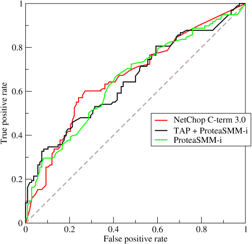
Above: Example of a ROC curve

First, the definitions. A ROC curve plots the performance of a binary classifier under various threshold settings; this is measured by true positive rate and false positive rate. If your classifier predicts “true” more often, it will have more true positives (good) but also more false positives (bad). If your classifier is more conservative, predicting “true” less often, it will have fewer false positives but fewer true positives as well. The ROC curve is a graphical representation of this tradeoff.

A perfect classifier has a 100% true positive rate and 0% false positive rate, so its ROC curve passes through the upper left corner of the square. A completely random classifier (ie: predicting “true” with probability p and “false” with probability 1-p for all inputs) will by random chance correctly classify proportion p of the actual true values and incorrectly classify proportion p of the false values, so its true and false positive rates are both p. Therefore, a completely random classifier’s ROC curve is a straight line through the diagonal of the plot.

The AUC (Area Under Curve) is the area enclosed by the ROC curve. A perfect classifier has AUC = 1 and a completely random classifier has AUC = 0.5. Usually, your model will score somewhere in between. The range of possible AUC values is [0, 1]. However, if your AUC is below 0.5, that means you can invert all the outputs of your classifier and get a better score, so you did something wrong.

The Gini Coefficient is 2*AUC – 1, and its purpose is to normalize the AUC so that a random classifier scores 0, and a perfect classifier scores 1. The range of possible Gini coefficient scores is [-1, 1]. If you search for “Gini Coefficient” on Google, you will find a closely related concept from economics that measures wealth inequality within a country.

---

Why do we care about AUC, why not just score by percentage accuracy?

AUC is good for classification problems with a class imbalance. Suppose the task is to detect dementia from speech, and 99% of people don’t have dementia and only 1% do. Then you can submit a classifier that always outputs “no dementia”, and that would achieve 99% accuracy. It would seem like your 99% accurate classifier is pretty good, when in fact it is completely useless. Using AUC scoring, your classifier would score 0.5.

In many classification problems, the cost of a false positive is different from the cost of a false negative. For example, it is worse to falsely imprison an innocent person than to let a guilty criminal get away, which is why our justice system assumes you’re innocent until proven guilty, and not the other way around. In a classification system, we would use a threshold rule, where everything above a certain probability is treated as 1, and everything below is treated as 0. However, deciding on where to draw the line requires weighing the cost of a false positive versus a false negative — this depends on external factors and has nothing to do with the classification problem.

AUC scoring lets us evaluate models independently of the threshold. This is why AUC is so popular in Kaggle: it enables competitors to focus on developing a good classifier without worrying about choosing the threshold, and let the organizers choose the threshold later.

(Note: This isn’t quite true — a classifier can sometimes be better at certain thresholds and worse at other thresholds. Sometimes it’s necessary to combine classifiers to get the best one for a particular threshold. Details in the paper linked at the end of this post.)

---

Next, here’s a mix of useful properties to know when working with ROC curves and AUC scoring.

AUC is not directly comparable to accuracy, precision, recall, or F1-score. If your model is achieving 0.65 AUC, it’s incorrect to interpret that as “65% accurate”. The reason is that AUC exists independently of a threshold and is immune to class imbalance, whereas accuracy / precision / recall / F1-score do require you picking a threshold, so you’re measuring two different things.

Only relative order matters for AUC score. When computing ROC AUC, we predict a probability for each data point, sort the points by predicted probability, and evaluate how close is it from a perfect ordering of the points. Therefore, AUC is invariant under scaling, or any transformation that preserves relative order. For example, predicting [0.03, 0.99, 0.05, 0.06] is the same as predicting [0.15, 0.92, 0.89, 0.91] because the relative ordering for the 4 items is the same in both cases.

A corollary of this is we can’t treat outputs of an AUC-optimized model as the likelihood that it’s true. Some models may be poorly calibrated (eg: its output is always between 0.3 and 0.32) but still achieve a good AUC score because its relative ordering is correct. This is something to look out for when blending together predictions of different models.

That’s my summary of the most important properties to know about ROC curves. There’s more that I haven’t talked about, like how to compute AUC score. If you’d like to learn more, I’d recommend reading “An introduction to ROC analysis” by Tom Fawcett.

I trained a neural network to describe pictures and it’s hilariously bad

This month, I’ve been working on a neural network to describe in a sentence what’s happening in a picture, otherwise known as image captioning. My model roughly follows the architecture outlined in the paper “Show and Tell: A Neural Image Caption Generator” by Vinyals et al., 2014.

A high level overview: the neural network first uses a convolutional neural network to turn the picture into an abstract representation. Then, it uses this representation as the initial hidden state of a recurrent neural network or LSTM, which generates a natural language sentence. This type of neural network is called an encoder-decoder network and is commonly used for a lot of NLP tasks like machine translation.

Above: Encoder-decoder image captioning neural network (Figure 1 of paper)

When I first encountered LSTMs, I was really confused about how they worked, and how to train them. If your output is a sequence of words, what is your loss function and how do you backpropagate it? In fact, the training and inference passes of an LSTM are quite different. In this blog post, I’ll try to explain this difference.

Above: Training procedure for caption LSTM, given known image and caption

During training mode, we train the neural network to minimize perplexity of the image-caption pair. Perplexity measures how the likelihood that the neural network would generate the given caption when it sees the given image. If we’re training it to output the caption “a cute cat”, the perplexity is:

P(“a” | image) *

P(“cute” | image, “a”) *

P(“cat” | image, “a”, “cute”) * …

(Note: for numerical stability reasons, we typically work with sums of negative log likelihoods rather than products of likelihood probabilities, so perplexity is actually the negative log of that whole thing)

After passing the whole sequence through the LSTM one word at a time, we get a single value, the perplexity, which we can minimize using backpropagation and gradient descent. As perplexity gets lower and lower, the LSTM is more likely to produce similar captions to the ground truth when it sees a similar image. This is how the network learns to caption images.

Above: Inference procedure for caption LSTM, given only the image but no caption

During inference mode, we repeatedly sample the neural network, one word at a time, to produce a sentence. On each step, the LSTM outputs a probability distribution for the next word, over the entire vocabulary. We pick the highest probability word, add it to the caption, and feed it back into the LSTM. This is repeated until the LSTM generates the end marker. Hopefully, if we trained it properly, the resulting sentence will actually describe what’s happening in the picture.

This is the main idea of the paper, and I omitted a lot details. I encourage you to read the paper for the finer points.

---

I implemented the model using PyTorch and trained it using the MS COCO dataset, which contains about 80,000 images of common objects and situations, and each image is human annotated with 5 captions.

To speed up training, I used a pretrained VGG16 convnet, and pretrained GloVe word embeddings from SpaCy. Using lots of batching, the Adam optimizer, and a Titan X GPU, the neural network trains in about 4 hours. It’s one thing to understand how it works on paper, but watching it actually spit out captions for real images felt like magic.

Above: How I felt when I got this working

How are the results? For some of the images, the neural network does great:

“A train is on the tracks at a station”

“A woman is holding a cat in her arms”

Other times the neural network gets confused, with amusing results:

“A little girl holding a stuffed animal in her hand”

“A baby laying on a bed with a stuffed animal”

“A dog is running with a frisbee in its mouth”

I’d say we needn’t worry about the AI singularity anytime soon 🙂

The original paper has some more examples of correct and incorrect captions that might be generated. Newer models also made improvements to generate more accurate captions: for example, adding a visual attention mechanism improved the results a bit. However, the state-of-the-art models still fall short on human performance; they often make mistakes when describing pictures with objects in unusual configurations.

This is a work in progress; source code is on Github here.

Publishing Negative Results in Machine Learning is like Proving Dragons don’t Exist

I’ve been reading a lot of machine learning papers lately, and one thing I’ve noticed is that the vast majority of papers report positive results — “we used method X on problem Y, and beat the state-of-the-art results”. Very rarely do you see a paper that reports that something doesn’t work.

The result is publication bias — if we only publish the results of experiments that succeed, even statistically significant results could be due to random chance, rather than anything actually significant happening. Many areas of science are facing a replication crisis, where published research cannot be replicated.

There is some community discussion of encouraging more negative paper submissions, but as of now, negative results are rarely publishable. If you attempt an experiment but don’t get the results you expected, your best hope is to try a bunch of variations of the experiment until you get some positive result (perhaps on a special case of the problem), after which you pretend the failed experiments never happened. With few exceptions, any positive result is better than a negative result, like “we tried method X on problem Y, and it didn’t work”.

Why publication bias is not so bad

I just described a cynical view of academia, but actually, there’s a good reason why the community prefers positive results. Negative results are simply not very useful, and contribute very little to human knowledge.

Now why is that? When a new paper beats the state-of-the-art results on a popular benchmark, that’s definite proof that the method works. The converse is not true. If your model fails to produce good results, it could be due to a number of reasons:

• Your dataset is too small / too noisy
• You’re using the wrong batch size / activation function / regularization
• You’re using the wrong loss function / wrong optimizer
• Your model is overfitting
• You have a bug in your code
• …

Above: Only when everything is correct will you get positive results; many things can cause a model to fail. (Source)

So if you try method X on problem Y and it doesn’t work, you gain very little information. In particular, you haven’t proved that method X cannot work. Sure, you found that your specific setup didn’t work, but have you tried making modification Z? Negative results in machine learning are rare because you can’t possibly anticipate all possible variations of your method and convince people that all of them won’t work.

Searching for dragons

Suppose we’re scientists attending the International Conference of Flying Creatures (ICFC). Somebody mentioned it would be nice if we had dragons. Dragons are useful. You could do all sorts of cool stuff with a dragon, like ride it into battle.

“But wait!” you exclaim: “Dragons don’t exist!”

I glance at you questioningly: “How come? We haven’t found one yet, but we’ll probably find one soon.”

Your intuition tells you dragons shouldn’t exist, but you can’t articulate a convincing argument why. So you go home, and you and your team of grad students labor for a few years and publish a series of papers:

• “We looked for dragons in China and we didn’t find any”
• “We looked for dragons in Europe and we didn’t find any”
• “We looked for dragons in North America and we didn’t find any”
• …

Eventually, the community is satisfied that dragons probably don’t exist, for if they did, someone would have found one by now. But a few scientists still harbor the possibility that there may be dragons lying around in a remote jungle somewhere. We just don’t know for sure.

This remains the state of things for a few years until a colleague publishes a breakthrough result:

• “Here’s a calculation that shows that any dragon with a wing span longer than 5 meters will collapse under its own weight”

You read the paper, and indeed, the logic is impeccable. This settles the matter once and for all: dragons don’t exist (or at least the large, flying sort of dragons).

When negative results are actually publishable

The research community dislikes negative results because they don’t prove a whole lot — you can have a lot of negative results and still not be sure that the task is impossible. In order for a negative result to be valuable, it needs to present a convincing argument why the task is impossible, and not just a list of experiments that you tried that failed.

This is difficult, but it can be done. Let me give an example from computational linguistics. Recurrent neural networks (RNNs) can, in theory, compute any function defined over a sequence. In practice, however, they had difficulty remembering long-term dependencies. Attempts to train RNNs using gradient descent ran into numerical difficulties known as the vanishing / exploding gradient problem.

Then, Bengio et al. (1994) formulated a mathematical model of an RNN as an iteratively applied function. Using ideas from dynamical systems theory, they showed that as the input sequence gets longer and longer, the result is more and more sensitive to noise. The details are technical, but the gist of it is that under some reasonable assumptions, training RNNs using gradient descent is impossible. This is a rare example of a negative result in machine learning — it’s an excellent paper and I’d recommend reading it.

Above: A Long Short Term Memory (LSTM) network handles long term dependencies by adding a memory cell (Source)

Soon after the vanishing gradient problem was understood, researchers invented the LSTM (Hochreiter and Schmidhuber, 1997). Since training RNNs with gradient descent was hopeless, they added a ‘latching’ mechanism that allows state to persist through many iterations, thus avoiding the vanishing gradient problem. Unlike plain RNNs, LSTMs can handle long term dependencies and can be trained with gradient descent; they are among the most ubiquitous deep learning architectures in NLP today.

---

After reading the breakthrough dragon paper, you pace around your office, thinking. Large, flying dragons can’t exist after all, as they would collapse under their own weight — but what about smaller, non-flying dragons? Maybe we’ve been looking for the wrong type of dragons all along? Armed with new knowledge, you embark on a new search…

Above: Komodo Dragon, Indonesia

…and sure enough, you find one 🙂