Clustering Autoencoders: Comparing DEC and DCN

Deep autoencoders are a good way to learn representations and structure from unlabelled data. There are many variations, but the main idea is simple: the network consists of an encoder, which converts the input into a low-dimensional latent vector, and a decoder, which reconstructs the original input. Then, the latent vector captures the most essential information in the input.

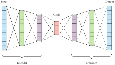
Above: Diagram of a simple autoencoder (Source)

One of the uses of autoencoders is to discover clusters of similar instances in an unlabelled dataset. In this post, we examine some ways of clustering with autoencoders. That is, we are given a dataset and K, the number of clusters, and need to find a low-dimensional representation that contains K clusters.

Problem with Naive Method

An naive and obvious solution is to take the autoencoder, and run K-means on the latent points generated by the encoder. The problem is that the autoencoder is only trained to reconstruct the input, with no constraints on the latent representation, and this may not produce a representation suitable for K-means clustering.

Above: Failure example with naive autoencoder clustering — K-means fails to find the appropriate clusters

Above is an example from one of my projects. The left diagram shows the hidden representation, and the four classes are generally well-separated. This representation is reasonable and the reconstruction error is low. However, when we run K-means (right), it fails spectacularly because the two latent dimensions are highly correlated.

Thus, our autoencoder can’t trivially be used for clustering. Fortunately, there’s been some research in clustering autoencoders; in this post, we study two main approaches: Deep Embedded Clustering (DEC), and Deep Clustering Network (DCN).

DEC: Deep Embedded Clustering

DEC was proposed by Xie et al. (2016), perhaps the first model to use deep autoencoders for clustering. The training consists of two stages. In the first stage, we initialize the autoencoder by training it the usual way, without clustering. In the second stage, we throw away the decoder, and refine the encoder to produce better clusters with a “cluster hardening” procedure.

Above: Diagram of DEC model (Xie et al., 2016)

Let’s examine the second stage in more detail. After training the autoencoder, we run K-means on the hidden layer to get the initial centroids . The assumption is the initial cluster assignments are mostly correct, but we can still refine them to be more distinct and separated.

First, we soft-assign each latent point to the cluster centroids using the Student’s t-distribution as a kernel:

In the paper, they fix (the degrees of freedom), so the above can be simplified to:

Next, we define an auxiliary distribution P by:

where is the soft cluster frequency of cluster j. Intuitively, squaring draws the probability distribution closer to the centroids.

Above: The auxiliary distribution P is derived from Q, but more concentrated around the centroids

Finally, we define the objective to minimize as the KL divergence between the soft assignment distribution Q and the auxiliary distribution P:

Using standard backpropagation and stochastic gradient descent, we can train the encoder to produce latent points to minimize the KL divergence L. We repeat this until the cluster assignments are stable.

DCN: Deep Clustering Network

DCN was proposed by Yang et al. (2017) at around the same time as DEC. Similar to DEC, it initializes the network by training the autoencoder to only reconstruct the input, and initialize K-means on the hidden representations. But unlike DEC, it then alternates between training the network and improving the clusters, using a joint loss function.

Above: Diagram of DCN model (Yang et al., 2017)

We define the optimization objective as a combination of reconstruction error (first term below) and clustering error (second term below). There’s a hyperparameter to balance the two terms:

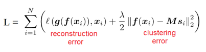
This function is complicated and difficult to optimize directly. Instead, we alternate between fixing the clusters while updating the network parameters, and fixing the network while updating the clusters. When we fix the clusters (centroid locations and point assignments), then the gradient of L with respect to the network parameters can be computed with backpropagation.

Next, when we fix the network parameters, we can update the cluster assignments and centroid locations. The paper uses a rolling average trick to update the centroids in an online manner, but I won’t go into the details here. The algorithm as presented in the paper looks like this:

Comparisons and Further Reading

To recap, DEC and DCN are both models to perform unsupervised clustering using deep autoencoders. When evaluated on MNIST clustering, their accuracy scores are comparable. For both models, the scores depend a lot on initialization and hyperparameters, so it’s hard to say which is better.

One theoretical disadvantage of DEC is that in the cluster refinement phase, there is no longer any reconstruction loss to force the representation to remain reasonable. So the theoretical global optimum can be achieved trivially by mapping every input to the zero vector, but this does not happen in practice when using SGD for optimization.

Recently, there have been lots of innovations in deep learning for clustering, which I won’t be covering in this post; the review papers by Min et al. (2018) and Aljalbout et al. (2018) provide a good overview of the topic. Still, DEC and DCN are strong baselines for the clustering task, which newer models are compared against.

References

1. Xie, Junyuan, Ross Girshick, and Ali Farhadi. “Unsupervised deep embedding for clustering analysis.” International conference on machine learning. 2016.
2. Yang, Bo, et al. “Towards k-means-friendly spaces: Simultaneous deep learning and clustering.” Proceedings of the 34th International Conference on Machine Learning-Volume 70. JMLR. org, 2017.
3. Min, Erxue, et al. “A survey of clustering with deep learning: From the perspective of network architecture.” IEEE Access 6 (2018): 39501-39514.
4. Aljalbout, Elie, et al. “Clustering with deep learning: Taxonomy and new methods.” arXiv preprint arXiv:1801.07648 (2018).

Deep Learning for NLP: SpaCy vs PyTorch vs AllenNLP

Deep neural networks have become really popular nowadays, producing state-of-the-art results in many areas of NLP, like sentiment analysis, text summarization, question answering, and more. In this blog post, we compare three popular NLP deep learning frameworks: SpaCy, PyTorch, and AllenNLP: what are their advantages, disadvantages, and use cases.

SpaCy

Pros: easy to use, very fast, ready for production

Cons: not customizable, internals are opaque

SpaCy is a mature and batteries-included framework that comes with prebuilt models for common NLP tasks like classification, named entity recognition, and part-of-speech tagging. It’s very easy to train a model with your data: all the gritty details like tokenization and word embeddings are handled for you. SpaCy is written in Cython which makes it faster than a pure Python implementation, so it’s ideal for production.

The design philosophy is the user should only worry about the task at hand, and not the underlying details. If a newer and more accurate model comes along, SpaCy can update itself to use the improved model, and the user doesn’t need to change anything. This is good for getting a model up and running quickly, but leaves little room for a NLP practitioner to customize the model if the task doesn’t exactly match one of SpaCy’s prebuilt models. For example, you can’t build a classifier that takes both text, numerical, and image data at the same time to produce a classification.

PyTorch

Pros: very customizable, widely used in deep learning research

Cons: fewer NLP abstractions, not optimized for speed

PyTorch is a deep learning framework by Facebook, popular among researchers for all kinds of DL models, like image classifiers or deep reinforcement learning or GANs. It uses a clear and flexible design where the model architecture is defined with straightforward Python code (rather than TensorFlow’s computational graph design).

NLP-specific functionality, like tokenization and managing word embeddings, are available in torchtext. However, PyTorch is a general purpose deep learning framework and has relatively few NLP abstractions compared to SpaCy and AllenNLP, which are designed for NLP.

AllenNLP

Pros: excellent NLP functionality, designed for quick prototyping

Cons: not yet mature, not optimized for speed

AllenNLP is built on top of PyTorch, designed for rapid prototyping NLP models for research purposes. It supports a lot of NLP functionality out-of-the-box, like text preprocessing and character embeddings, and abstracts away the training loop (whereas in PyTorch you have to write the training loop yourself). Currently, AllenNLP is not yet at a 1.0 stable release, but looks very promising.

Unlike PyTorch, AllenNLP’s design decouples what a model “does” from the architectural details of “how” it’s done. For example, a Seq2VecEncoder is any component that takes a sequence of vectors and outputs a single vector. You can use GloVe embeddings and average them, or you can use an LSTM, or you can put in a CNN. All of these are Seq2VecEncoders so you can swap them out without affecting the model logic.

The talk “Writing code for NLP Research” presented at EMNLP 2018 gives a good overview of AllenNLP’s design philosophy and its differences from PyTorch.

Which is the best framework?

It depends on how much you care about flexibility, ease of use, and performance.

• If your task is fairly standard, then SpaCy is the easiest to get up and running. You can train a model using a small amount of code, you don’t have to think about whether to use a CNN or RNN, and the API is clearly documented. It’s also well optimized to deploy to production.
• AllenNLP is the best for research prototyping. It supports all the bells and whistles that you’d include in your next research paper, and encourages you to follow the best practices by design. Its functionality is a superset of PyTorch’s, so I’d recommend AllenNLP over PyTorch for all NLP applications.

There’s a few runner-ups that I will mention briefly:

• NLTK / Stanford CoreNLP / Gensim are popular libraries for NLP. They’re good libraries, but they don’t do deep learning, so they can’t be directly compared here.
• Tensorflow / Keras are also popular for research, especially for Google projects. Tensorflow is the only framework supported by Google’s TPUs, and it also has better multi-GPU support than PyTorch. However, multi-GPU setups are relatively uncommon in NLP, and furthermore, its computational graph model is harder to debug than PyTorch’s model, so I don’t recommend it for NLP.
• PyText is a new framework by Facebook, also built on top of PyTorch. It defines a network using pre-built modules (similar to Keras) and supports exporting models to Caffe to be faster in production. However, it’s very new (only released earlier this month) and I haven’t worked with it myself to form an opinion about it yet.

That’s all, let me know if there’s any that I’ve missed!

I trained a neural network to describe images, then I gave it dementia

This blog post is a summary of my work from earlier this year: Dropout during inference as a model for neurological degeneration in an image captioning network.

For a long time, deep learning has had an interesting connection to neuroscience. The definition of the neuron in neural networks was inspired by early models of the neuron. Later, convolutional neural networks were inspired by the structure of neurons in the visual cortex. Many other models also drew inspiration from how the brain functions, like visual attention which replicated how humans looked at different areas of an image when interpreting it.

The connection was always a loose and superficial, however. Despite advances in neuroscience about better models of neurons, these never really caught on among deep learning researchers. Real neurons obviously don’t learn by gradient back-propagation and stochastic gradient descent.

In this work, we study how human neurological degeneration can have a parallel in the universe of deep neural networks. In humans, neurodegeneration can occur by several mechanisms, such as Alzheimer’s disease (which affects connections between individual neurons) or stroke (in which large sections of brain tissue die). The effect of Alzheimer’s disease is dementia, where language, motor, and other cognitive abilities gradually become impaired.

To simulate this effect, we give our neural network a sort of dementia, by interfering with connections between neurons using a method called dropout.

Yup, this probably puts me high up on the list of humans to exact revenge in the event of an AI apocalypse.

The Model

We started with an encoder-decoder style image captioning neural network (described in this post), which looks at an image and outputs a sentence that describes it. This is inspired by a picture description task that we give to patients suspected of having dementia: given a picture, describe it in as much detail as possible. Patients with dementia typically exhibit patterns of language different from healthy patients, which we can detect using machine learning.

To simulate neurological degeneration in the neural network, we apply dropout in the inference mode, which randomly selects a portion of the neurons in a layer and sets their outputs to zero. Dropout is a common technique during training to regularize neural networks to prevent overfitting, but usually you turn it off during evaluation for the best possible accuracy. To our knowledge, nobody’s experimented with applying dropout in the evaluation stage in a language model before.

We train the model using a small amount of dropout, then apply a larger amount of dropout during inference. Then, we evaluate the quality of the sentences produced by BLEU-4 and METEOR metrics, as well as sentence length and similarity of vocabulary distribution to the training corpus.

Results

When we applied dropout during inference, the accuracy of the captions (measured by BLEU-4 and METEOR) decreased with more dropout. However, the vocabulary generated was more diverse, and the word frequency distribution was more similar (measured by KL-divergence to the training set) when a moderate amount of dropout was applied.

When the dropout was too high, the model degenerated into essentially generating random words. Here are some examples of sentences that were generated, at various levels of dropout:

Qualitatively, the effects of dropout seemed to cause two types of errors:

• Caption starts out normally, then repeats the same word several times: “a small white kitten with red collar and yellow chihuahua chihuahua chihuahua”
• Caption starts out normally, then becomes nonsense: “a man in a baseball bat and wearing a uniform helmet and glove preparing their handles won while too frown”

This was not that similar to speech produced by people with Alzheimer’s, but kind of resembled fluent aphasia (caused by damage to the part of the brain responsible for understanding language).

Challenges and Difficulties

Excited with our results, we submitted the paper to EMNLP 2018. Unfortunately, our paper was rejected. Despite the novelty of our approach, the reviewers pointed out that our work had some serious drawbacks:

1. Unclear connection to neuroscience. Adding dropout during inference mode has no connections to any biological models of what happens to the brain during atrophy.
2. Only superficial resemblance to aphasic speech. A similar result could have been generated by sampling words randomly from a dictionary, without any complicated RNN models.
3. Not really useful for anything. We couldn’t think of any situations where this model would be useful, such as detecting aphasia.

We decided that there was no way around these roadblocks, so we scrapped the idea, put the paper up on arXiv and worked on something else.

For more technical details, refer to our paper:

• Li, Bai, Ran Zhang, and Frank Rudzicz. “Dropout during inference as a model for neurological degeneration in an image captioning network.” arXiv preprint arXiv:1808.03747(2018).

I trained a neural network to describe pictures and it’s hilariously bad

This month, I’ve been working on a neural network to describe in a sentence what’s happening in a picture, otherwise known as image captioning. My model roughly follows the architecture outlined in the paper “Show and Tell: A Neural Image Caption Generator” by Vinyals et al., 2014.

A high level overview: the neural network first uses a convolutional neural network to turn the picture into an abstract representation. Then, it uses this representation as the initial hidden state of a recurrent neural network or LSTM, which generates a natural language sentence. This type of neural network is called an encoder-decoder network and is commonly used for a lot of NLP tasks like machine translation.

Above: Encoder-decoder image captioning neural network (Figure 1 of paper)

When I first encountered LSTMs, I was really confused about how they worked, and how to train them. If your output is a sequence of words, what is your loss function and how do you backpropagate it? In fact, the training and inference passes of an LSTM are quite different. In this blog post, I’ll try to explain this difference.

Above: Training procedure for caption LSTM, given known image and caption

During training mode, we train the neural network to minimize perplexity of the image-caption pair. Perplexity measures how the likelihood that the neural network would generate the given caption when it sees the given image. If we’re training it to output the caption “a cute cat”, the perplexity is:

P(“a” | image) *

P(“cute” | image, “a”) *

P(“cat” | image, “a”, “cute”) * …

(Note: for numerical stability reasons, we typically work with sums of negative log likelihoods rather than products of likelihood probabilities, so perplexity is actually the negative log of that whole thing)

After passing the whole sequence through the LSTM one word at a time, we get a single value, the perplexity, which we can minimize using backpropagation and gradient descent. As perplexity gets lower and lower, the LSTM is more likely to produce similar captions to the ground truth when it sees a similar image. This is how the network learns to caption images.

Above: Inference procedure for caption LSTM, given only the image but no caption

During inference mode, we repeatedly sample the neural network, one word at a time, to produce a sentence. On each step, the LSTM outputs a probability distribution for the next word, over the entire vocabulary. We pick the highest probability word, add it to the caption, and feed it back into the LSTM. This is repeated until the LSTM generates the end marker. Hopefully, if we trained it properly, the resulting sentence will actually describe what’s happening in the picture.

This is the main idea of the paper, and I omitted a lot details. I encourage you to read the paper for the finer points.

---

I implemented the model using PyTorch and trained it using the MS COCO dataset, which contains about 80,000 images of common objects and situations, and each image is human annotated with 5 captions.

To speed up training, I used a pretrained VGG16 convnet, and pretrained GloVe word embeddings from SpaCy. Using lots of batching, the Adam optimizer, and a Titan X GPU, the neural network trains in about 4 hours. It’s one thing to understand how it works on paper, but watching it actually spit out captions for real images felt like magic.

Above: How I felt when I got this working

How are the results? For some of the images, the neural network does great:

“A train is on the tracks at a station”

“A woman is holding a cat in her arms”

Other times the neural network gets confused, with amusing results:

“A little girl holding a stuffed animal in her hand”

“A baby laying on a bed with a stuffed animal”

“A dog is running with a frisbee in its mouth”

I’d say we needn’t worry about the AI singularity anytime soon 🙂

The original paper has some more examples of correct and incorrect captions that might be generated. Newer models also made improvements to generate more accurate captions: for example, adding a visual attention mechanism improved the results a bit. However, the state-of-the-art models still fall short on human performance; they often make mistakes when describing pictures with objects in unusual configurations.

This is a work in progress; source code is on Github here.

Publishing Negative Results in Machine Learning is like Proving Dragons don’t Exist

I’ve been reading a lot of machine learning papers lately, and one thing I’ve noticed is that the vast majority of papers report positive results — “we used method X on problem Y, and beat the state-of-the-art results”. Very rarely do you see a paper that reports that something doesn’t work.

The result is publication bias — if we only publish the results of experiments that succeed, even statistically significant results could be due to random chance, rather than anything actually significant happening. Many areas of science are facing a replication crisis, where published research cannot be replicated.

There is some community discussion of encouraging more negative paper submissions, but as of now, negative results are rarely publishable. If you attempt an experiment but don’t get the results you expected, your best hope is to try a bunch of variations of the experiment until you get some positive result (perhaps on a special case of the problem), after which you pretend the failed experiments never happened. With few exceptions, any positive result is better than a negative result, like “we tried method X on problem Y, and it didn’t work”.

Why publication bias is not so bad

I just described a cynical view of academia, but actually, there’s a good reason why the community prefers positive results. Negative results are simply not very useful, and contribute very little to human knowledge.

Now why is that? When a new paper beats the state-of-the-art results on a popular benchmark, that’s definite proof that the method works. The converse is not true. If your model fails to produce good results, it could be due to a number of reasons:

• Your dataset is too small / too noisy
• You’re using the wrong batch size / activation function / regularization
• You’re using the wrong loss function / wrong optimizer
• Your model is overfitting
• You have a bug in your code
• …

Above: Only when everything is correct will you get positive results; many things can cause a model to fail. (Source)

So if you try method X on problem Y and it doesn’t work, you gain very little information. In particular, you haven’t proved that method X cannot work. Sure, you found that your specific setup didn’t work, but have you tried making modification Z? Negative results in machine learning are rare because you can’t possibly anticipate all possible variations of your method and convince people that all of them won’t work.

Searching for dragons

Suppose we’re scientists attending the International Conference of Flying Creatures (ICFC). Somebody mentioned it would be nice if we had dragons. Dragons are useful. You could do all sorts of cool stuff with a dragon, like ride it into battle.

“But wait!” you exclaim: “Dragons don’t exist!”

I glance at you questioningly: “How come? We haven’t found one yet, but we’ll probably find one soon.”

Your intuition tells you dragons shouldn’t exist, but you can’t articulate a convincing argument why. So you go home, and you and your team of grad students labor for a few years and publish a series of papers:

• “We looked for dragons in China and we didn’t find any”
• “We looked for dragons in Europe and we didn’t find any”
• “We looked for dragons in North America and we didn’t find any”
• …

Eventually, the community is satisfied that dragons probably don’t exist, for if they did, someone would have found one by now. But a few scientists still harbor the possibility that there may be dragons lying around in a remote jungle somewhere. We just don’t know for sure.

This remains the state of things for a few years until a colleague publishes a breakthrough result:

• “Here’s a calculation that shows that any dragon with a wing span longer than 5 meters will collapse under its own weight”

You read the paper, and indeed, the logic is impeccable. This settles the matter once and for all: dragons don’t exist (or at least the large, flying sort of dragons).

When negative results are actually publishable

The research community dislikes negative results because they don’t prove a whole lot — you can have a lot of negative results and still not be sure that the task is impossible. In order for a negative result to be valuable, it needs to present a convincing argument why the task is impossible, and not just a list of experiments that you tried that failed.

This is difficult, but it can be done. Let me give an example from computational linguistics. Recurrent neural networks (RNNs) can, in theory, compute any function defined over a sequence. In practice, however, they had difficulty remembering long-term dependencies. Attempts to train RNNs using gradient descent ran into numerical difficulties known as the vanishing / exploding gradient problem.

Then, Bengio et al. (1994) formulated a mathematical model of an RNN as an iteratively applied function. Using ideas from dynamical systems theory, they showed that as the input sequence gets longer and longer, the result is more and more sensitive to noise. The details are technical, but the gist of it is that under some reasonable assumptions, training RNNs using gradient descent is impossible. This is a rare example of a negative result in machine learning — it’s an excellent paper and I’d recommend reading it.

Above: A Long Short Term Memory (LSTM) network handles long term dependencies by adding a memory cell (Source)

Soon after the vanishing gradient problem was understood, researchers invented the LSTM (Hochreiter and Schmidhuber, 1997). Since training RNNs with gradient descent was hopeless, they added a ‘latching’ mechanism that allows state to persist through many iterations, thus avoiding the vanishing gradient problem. Unlike plain RNNs, LSTMs can handle long term dependencies and can be trained with gradient descent; they are among the most ubiquitous deep learning architectures in NLP today.

---

After reading the breakthrough dragon paper, you pace around your office, thinking. Large, flying dragons can’t exist after all, as they would collapse under their own weight — but what about smaller, non-flying dragons? Maybe we’ve been looking for the wrong type of dragons all along? Armed with new knowledge, you embark on a new search…

Above: Komodo Dragon, Indonesia

…and sure enough, you find one 🙂

Kaggle Speech Recognition Challenge

For the past few weeks, I’ve been working on the TensorFlow Speech Recognition Challenge on Kaggle. The task is to recognize a one-second audio clip, where the clip contains one of a small number of words, like “yes”, “no”, “stop”, “go”, “left”, and “right”.

In general, speech recognition is a difficult problem, but it’s much easier when the vocabulary is limited to a handful of words. We don’t need to use complicated language models to detect phonemes, and then string the phonemes into words, like Kaldi does for speech recognition. Instead, a convolutional neural network works quite well.

First Steps

The dataset consists of about 64000 audio files which have already been split into training / validation / testing sets. You are then asked to make predictions on about 150000 audio files for which the labels are unknown.

Actually, this dataset had already been published in academic literature, and people published code to solve the same problem. I started with GCommandPytorch by Yossi Adi, which implements a speech recognition CNN in Pytorch.

The first step that it does is convert the audio file into a spectrogram, which is an image representation of sound. This is easily done using LibRosa.

Above: Sample spectrograms of “yes” and “no”

Now we’ve converted the problem to an image classification problem, which is well studied. To an untrained human observer, all the spectrograms may look the same, but neural networks can learn things that humans can’t. Convolutional neural networks work very well for classifying images, for example VGG16:

Above: A Convolutional Neural Network (LeNet). VGG16 is similar, but has even more layers.

For more details about this approach, refer to these papers:

1. Convolutional Neural Networks for Small-footprint Keyword Spotting

2. Honk: A PyTorch Reimplementation of Convolutional Neural Networks for Keyword Spotting

Voice Activity Detection

You might ask: if somebody already implemented this, then what’s there left to do other than run their code? Well, the test data contains “silence” samples, which contain background noise but no human speech. It also has words outside the set we care about, which we need to label as “unknown”. The Pytorch CNN produces about 95% validation accuracy by itself, but the accuracy is much lower when we add these two additional requirements.

For silence detection, I first tried the simplest thing I could think of: taking the maximum absolute value of the waveform and decide it’s “silence” if the value is below a threshold. When combined with VGG16, this gets accuracy 0.78 on the leaderboard. This is a crude metric because sufficiently loud noise would be considered speech.

Next, I tried running openSMILE, which I use in my research to extract various acoustic features from audio. It implements an LSTM for voice activity detection: every 0.05 seconds, it outputs a probability that someone is talking. Combining the openSMILE output with the VGG16 prediction gave a score of 0.81.

More improvements

I tried a bunch of things to improve my score:

1. Fiddled around with the neural network hyperparameters which boosted my score to 0.85. Each epoch took about 10 minutes on a GPU, and the whole model takes about 2 hours to train. Somehow, Adam didn’t produce good results, and SGD with momentum worked better.
2. Took 100% of the data for training and used the public LB for validation (don’t do this in real life lol). This improved my score to 0.86.
3. Trained an ensemble 3 versions of the same neural network with same hyperparameters but different randomly initialized weights and took a majority vote to do prediction. This improved the score to 0.87. I would’ve liked to train more, but other people in my research group needed to use the GPUs.

---

In the end, the top scoring model had a score of 0.91, which beat my model by 4 percentage points. Although not enough to win a Kaggle medal, my model was in the top 15% of all submissions. Not bad!

My source code for the contest is available here.