Algorithmic Trading Hackathon

The name of the hackathon was Code B: UW Algorithmic Trading Competition. It was hosted by Bloomberg and various UW student groups. It’s a 17 hour hackathon where you “create the best trading platform completely from scratch”. As far as I know, this is the first time the hackathon has been run, and in this article I’m going to write about my experience.

We were allowed teams of up to three, but my roommate Andrei and I signed up as a team of two. Like myself, Andrei is also a CS major. Neither of us had any experience with trading stocks, or anything finance related, for that matter. When asked to choose a team name, we named ourselves team /dev/rand (implying that we were so bad that we’d be no better than a random number generator)

The hackathon was scheduled to start Friday evening, running through the night until noon the next day. The goal was to write a program to autonomously trade stocks over a 20 minute period, battling other programs to earn as much money as possible. The programs communicated by connecting to a central server on Bloomberg’s side, so we could use any programming language we wanted. It was decided that Andrei would come up with strategies, and I would implement them in Python.

Rules of the Game

The specifics of the API and mechanics of the game were not revealed until the official start of the hackathon. The 50-60 teams packed into an auditorium as the organizers started to explain the technical details.

The rules turned out to be fairly simple. The only actions allowed were to bid (attempt to purchase) on a stock for some price, or ask (attempt to sell) a stock for some price. If at any point someone’s bid is higher than someone else’s ask, the deal goes through and the stock changes hands.

Now all of this was fairly standard, but after this part, the rules diverged from real life. In order to encourage people to buy stocks (and not just hoard the initial money), each share of a stock paid dividends to its owner every second. And to prevent simply buying one stock and holding it for the entire duration, the dividends given out quickly diminishes the longer you own the stock.

This quirky dividends system turned out to be central to our strategy. Additionally, the differences from real stock markets meant that any previous experience with finance and stock trading was less useful — definitely a good thing for us because many of our competitors were seriously studying finance and we had no experience anyway.

And it begins!

After the rules presentation, the hackathon kicked off. It was slightly past 7pm, and very quickly you could see teams buying and selling stocks. We decided to take it slow, discussing strategies over dinner.

We started work around 8pm. I began writing code to parse the input, while Andrei worked on deciphering the rather cryptic specifications document. Although API specs were clear enough, they were (intentionally) vague about how the system behaved behind the scenes. There were many formulas with lots of variables, many of which we had no idea what they meant.

So we took an experimental approach. Tentatively we put in a bid for a few shares of Google stock — and our net worth immediately took a nosedive. But the stock rapidly generated dividends, and before long, our net worth recovered to what it was initially, and it kept on going up! The success was short lasted, however, as quickly the dampening effects of the dividends started to kick in, and our rate of return quickly diminished to near zero.

We tried again, buying a few shares of the Twitter stock. The same thing happened — our value went down, quickly recovered, then gradually leveled to 50 dollars more than we started with.

With this information, we formulated a rough strategy. We didn’t know how to predict which stocks will go up; neither did we have a plan for buying and selling stocks at a favorable rate. Instead, we would take advantage of a stock’s “golden period”, where the stock initially pays massive dividends. It was crucial to buy as quickly as possible, since the clock started ticking as soon as you own one share of the stock. So we use all our money to buy as many shares of the stock as possible, doesn’t matter what price. Now we wait as the golden period payout multiplied by our entire bankroll makes us rich. Then, a few minutes later, when the golden period runs out, we would slowly sell, iteratively lowering our asking price until we found a buyer.

Once we sold the last share of a stock, the dividend clock doesn’t immediately reset, it slowly regenerates. So if we wait a while, say 5 minutes, then buy back the stock, we get another brief golden period. Taking this one step further, we decided on a strategy that cycled through the 10 stocks: at any given point, we would hold at most 4 of them, while the other 6 were left to “recharge”.

I proceeded to code the algorithm, while Andrei analyzed the spec document and brainstormed ways to improve the strategy. From the equations in the spec, he came up with a formula to determine what stock generated the highest dividends. Every half hour, the scoreboard would reset, and by 3am, I was basically done, and our algorithm consistently came either first or second by the end of each round. Our algorithm worked beautifully, simultaneously juggling a bunch of different stocks, some buying, others slowly selling. We watched the scoreboard as we earned hundreds of dollars every minute, ending with a ridiculous amount of money by the time it reset.

It seemed at this point that a lot of the teams were having implementation issues, like connecting to the network and parsing input, and only a handful were making any money at all, so I was pretty happy with our results.

But at 4am, disaster struck. A new round started, and our algorithm instantly plummeted to the bottom of the leaderboard. Every time we bought or sold anything, we lost money, and none of it was coming back through dividends. What happened?? It turns out that the parameters were changed, so that a very low amount of dividends were paid for owning a stock, and the only profits were made by buying low and selling high. This meant that our whole strategy, which centered around maximizing dividends, was rendered useless.

What’s worse — I discovered a bug in my implementation where our stocks were not being cycled properly: it would sell a certain stock, then instantly buy back the same stock, which didn’t allow the dividends clock to reset, meaning no dividends. Also, by this point a lot of teams were flooding the network with requests, making any network call have a small chance of throwing an exception and crashing the whole thing entirely.

The network problem was easy to fix, but at 5am, I was really tired and had difficulty tracking down the bug that was causing it to buy back the same stock. Andrei suggested a new set of strategies for the “low dividends” scenario, but by now, I was too tired to implement another set of strategies. Instead, we tweaked various constants in our program to make it play more patiently and more predictably, so even in the worst case it would make marginal gains instead of finishing dead last. After 2 hours of debugging, we managed to track down the cycling bug.

It was 7am and I could hardly keep my eyes open so we found a couch and napped for two hours, until the mock competition began.

Mock Competition and final tweaking

At 9am, a few hours before the final competition, there was a mock competition which was meant to be identical to the final competition. There were three rounds: a high dividends scenario, a low dividends, and one in the middle.

We won the high dividends round hands down, unsurprisingly as our entire strategy was designed around this set of parameters in mind. In the low dividends round, we didn’t do as well, but thanks to careful tweaking, we still made a modest amount of money, coming in fifth. In the medium round, we got second place. This was enough to win the mock competition.

Now, let me give you a summary of our competition. Most of the teams increased gradually in net worth, with their score slowly increasing as they slowly accumulated dividends. We were confident that we could play the dividends game, so it didn’t trouble us too much. What was really troubling was a team called “vlad” (I don’t quite remember what their name was, but it ended with vlad). Instead of gradually gaining money a few dollars at a time, “vlad” remained at a constant net worth for a long time, then suddenly gain hundreds of dollars instantly. This meant that their algorithm operated completely differently from ours, and we had absolutely no explanation of what was going on.

It didn’t help that the formula for net worth was complicated and we didn’t fully understand it. Our net worth clearly increased when we did well, but it fluctuated wildly, sometimes dipping by hundreds of points when we made a large transaction, only to bounce back when dividends started rolling in.

The next few hours were fairly unproductive, since we had no more ideas on how to improve our algorithm. Although Andrei had some ideas on strategies for the low dividends game, after pulling an all-nighter I was in no shape to try implementing them.

The Final Game

It was soon time for the final competition, the cumulation of all our efforts. Having carefully noted down the parameters for the mock competition, we were ready to use this information to get every edge we could for the finals.

Round 1 was high dividends. We played with a highly aggressive set of parameters, dumping our bad stocks for very cheap in pursuit of the dividends regeneration. The early game was contentious, but by the 10 minute mark, we gained a solid lead over the competition and maintained the lead until the end. We won round 1, with “vlad” coming in third place.

Round 2 was low dividends. We deployed the patient strategy, which was less eager to dump anything, holding onto bad stocks until we get a good price for them, since there were little dividends to fight over anyway. We came fifth place, with “vlad” coming in fourth.

Round 3 was medium dividends. We started off uncertain — at the halfway mark we were still in the middle of the pack — but slowly we gained ground, and five minutes before the end, we were in third position. “vlad” was in first place, with a big enough lead that neither we nor the second place team were going to overtake him. But at this point, we knew that from our points in the first round, we only needed second place to beat “vlad” and win the competition — and with 3 minutes left on the clock, we overtook the second place team. We were going to win it!

Then, the whole scoreboard goes black.

It didn’t crash, no, it was the contest organizers’ tactic to increase suspense so the final winners are not known until the winners are announced. We waited anxiously as the final seconds ticked down, the organizers announcing fourth place, third place, UI award. We just needed second place in this round to win, if we get third place in this round, “vlad” beats us by a hair.

And the second place goes to… team /dev/rand. What? We stared in disbelief as we realize we lost to “vlad”.

Going home

Turns out that in the last 2 minutes of competition, we got overtaken by not one, but two teams. So we actually finished round 3 in fourth place.

Our prize for winning second place? A playstation 4 (worth ~450) and a parrot drone (worth ~100), and most importantly, the satisfaction of winning a finance competition without knowing the first thing about finance. Team “vlad” got two playstations and a drone (well, they could have taken all 3 playstations but they were nice enough to leave us one)

Big thanks to all the organizers and volunteers for keeping everything running smoothly!

If you’re interested, our source code is in a git repo here. It’s 400 lines of hackathon-level-bad python code.

What about real algo trading?

A natural question to ask is, can we get rich IRL with this algorithm? Answer is clearly no — we essentially gamed the system by greedily grabbing the golden period of dividends, a mechanic designed to encourage people to buy and sell stocks. Of course, in the real world, dividends don’t work like that.

Then other than this mechanic, how else is this competition different from real world algo trading? Unfortunately, I don’t know enough about this topic to answer that question.

Philosophically, I still don’t understand how it’s possible that they basically pull money out of thin air. I mean, a stock trader doesn’t intrinsically create value for society, but they get rich doing it? I don’t know.

Splitting utility costs between roommates is NP-Complete

Here’s an easy problem.

You live in a house with 4 people. For simplicity, I will call them Andrei, Bai, Darin, and Young. One person pays for electricity, another person pays for gas, another person pays for water, and the last person pays for internet. However, the utilities cost different amounts, and it is agreed that the total cost should be split equally.

It has come to the time to wrap up the bills. After tallying up the receipts, you find that Andrei has paid $650, Bai has paid $240, Darin has paid $190, and Young has paid $120. What transfers do you make to distribute the costs fairly?

Well that’s easy. Add up all the numbers and you find that the group paid $1200 in total. A quarter of that is $300 — that’s the amount each person should pay in the end. If you’ve already paid $240, then the difference, $60, is the amount you have to pay to compensate.

To see this even more clearly, let us define balance as the difference between what you’re supposed to pay and what you actually paid. From now on, I will use a negative balance to mean you paid more than you supposed to and you are owed money; a positive balance means you owe money to others.

In this case, it’s obvious how to balance the bills. Since Andrei is the only person with a negative balance, everyone simply transfers the correct sum of money to Andrei, problem solved.

But in general…

Being a computer science major, this left me wondering: what if I lived with 20 people? And what if, throughout the term, we lend each other money, so that multiple people have a negative balance, and multiple people have a positive balance? How do we solve this problem then?

For simplicity, from now on I will assume the preliminary calculations have been done, and we will work solely with the balance column. I will also assume that all values are integers.

One immediate observation is the balances always add up to 0. So given a list of integers than add up to 0, how do we find an efficient set of transfers to balance the bill?

What do we mean by efficient? Well, let’s explore several possibilities.

Roommate Problem, version 1

Given a list of balances that add up to 0, find the smallest number of transfers to balance the bill.

This seems at first glance to be the criterion we’re looking for. Writing cheques is a hassle, so we don’t want to write more than what is absolutely necessary.

But if you think about it, there’s a really cheap way to solve this problem:

Sort the list. Starting from the highest number, give all your money to the second highest number, repeat n-1 times.

Somehow this doesn’t feel very satisfying. If there are a lot of people, the people in the middle are going to be handling enormous amounts of money. Let’s try again.

Roommate Problem, version 2

Given a list of balances that add up to 0, minimize the total money transferred to balance the bill.

Perhaps what we really want is to minimize the money transferred? Maybe the bank charges $0.01 for each $1 you transfer?

Unfortunately, this problem can also be solved in a cheap way:

We don’t care how many transfers we make, so let’s just transfer $1 at a time! As long as we always transfer from positive to negative, it doesn’t matter how we do it, we’re always going to transfer a fixed amount of money. Let’s try again.

Roommate Problem, version 3

Given a list of balances that add up to 0, find the smallest set of transfers to balance the bill, with the limitation that transfers are only allowed from a positive to a negative balance.

This captures our intuition that a person should either be transferring money or receiving money, not both.

Version 3 doesn’t fall immediately to a cheap trick like its two predecessors. Instances of this problem can get pretty tricky at times — here are some examples of some optimal solutions:

I couldn’t come up with an efficient algorithm to solve this problem. The best I could come up with was a greedy algorithm:

Assume the input is [-8,-4,5,7]. On each step, look for the number with the least absolute value (-4). Without loss of generality, assume this number is negative. Then ‘zero’ this number by cancelling it with the smallest number on the other side — so transfer $4 from 5 to 4, giving us [-8,1,7]. Repeat this until all numbers are zero.

How bad is this algorithm? Let’s say there are M negative numbers and N positive numbers. Then this algorithm requires at most M+N-1 transfers, since each step zeroes at least one number, and the last step zeroes two numbers.

The optimal solution takes at least max(M,N) transfers. This proves that my greedy algorithm never takes more than 2 times the optimal number of transfers. Not too bad, but not great either.

Unable to progress any further, I asked around in the TopCoder forums. Surprisingly, I got an answer that hinted the problem was impossible to solve efficiently — it is NP-Complete!

NP-Complete by Reduction from SUBSET-SUM

To prove a problem can be solved efficiently, you simply describe an algorithm that solves the problem, then prove this algorithm is efficient. But how do you prove a problem cannot be solved efficiently?

There are certain problems in computer science that are known to be hard: one of them is the Subset Sum problem. Given a set of positive integers and a positive integer N, is it possible to find a subset that sums to exactly N? Return YES if this is possible, or NO otherwise.

For example, say our set is {3,5,7,8,11}. Can we make 16? The answer is YES, because 5+11=16. Can we make 17? The answer is NO — if you check all the possibilities, you discover that no subset sums to exactly 17.

We can leverage the fact that the Subset Sum problem is hard using a proof by contradiction. Assume that there exists some efficient algorithm to solve the Roommate problem. In the diagram, I symbolize it with a black box.

Assume there is also a converter routine: an easy way to convert an input for the Subset Sum problem into an input for the Roommate problem. I’ll get to the details of this converter shortly; right now, assume it exists.

Then combining the Roommate solver with the converter, we have created a Subset Sum solver! If the Roommate solver is efficient, then this Subset Sum solver is also efficient. But we know that no efficient Subset Sum solver exists. Ergo, no efficient Roommate solver exists either.

The only missing piece is to reduce an instance of the Subset Sum problem to an input to the Roommate problem.

Here’s how. For each number in your set, create a roommate with that number as a positive balance. Then create a roommate with a balance of -N (the number you’re trying to sum up to). Then create one final roommate with the exact balance so that all the numbers sum to 0.

Here’s the input for {3,5,7,8,11} and N=16:

There are 5 numbers in the set, and the Roommate solver finds a solution requiring 5 transfers.

By contrast, here’s the input for {3,5,7,8,11} and N=17:

The Roommate solver can’t do better than 6 transfers.

So to solve the Subset Sum problem, plug it into the Roommate solver and see how many transfers it outputs. If it outputs exactly 1 transfer for every element in your set, then output YES. Otherwise, if there are more transfers than elements in your set, output NO.

This proves that the Roommate problem is as least as hard as Subset Sum, so it’s NP-Complete.

Research in Existing Literature and Application to Biology

While researching for this blog post, I came upon this research paper titled “On the Minimum Common Integer Partition Problem” published in 2006 by Xin Cheng, Lan Liu, Zheng Liu, and Tao Jiang.

They investigate a problem they call Minimum Common Integer Partition (MCIP). Given two lists of integers, say [4,8] and [5,7], find the smallest common partition — in this case, [3,4,5].

Compare this to the Roommate problem with input [-4,-8,5,7], and it’s clear that the Roommate problem is identical to 2-MCIP. (The 2 just means we’re finding the smallest partition between 2 lists, the paper also investigates finding the smallest partition between more than 2 lists).

Skimming through this paper, it derives an algorithm similar to my greedy algorithm which approximates the problem by a factor of 2. Using more complicated techniques, it manages to produce an algorithm with a 5/4 approximation.

Doing a bit more searching, it turns out that a more recent paper by David Woodruff reduces the approximation ratio for 2-MCIP down to 1.228; an even better paper reduces it down to 1.125 using network flow techniques. At this point, I think I’m way too sidetracked from the original problem, so I didn’t investigate the details.

What surprised me more was that this research was motivated not by roommates sharing utilities, but by biologists studying genome sequences! Biology is not my area of expertise, so I won’t comment further on that. But I’ll leave you these slides (taken from a presentation by the above-mentioned David Woodruff):

So in short, we can’t solve the Roommate problem perfectly, but with cutting-edge algorithms, we can guarantee ourselves to be off by no more than 12.5%!

How to Write your own Minesweeper AI

A while ago, I wrote a minesweeper AI. I intended to publish a writeup, but due to university and life and exams, I never got around to writing it. But having just finished my Fall term, I have some time to write a decent overview of what I did.

Short 30 second video of the AI in action here:

How to Play Minesweeper

If you’re an experienced minesweeper player, you can probably skip this section. Otherwise, I’ll just give a quick overview of some basic strategies that we can use to solve an easy minesweeper game.

We start with a 10×10 Beginner’s grid, and click on a square in the middle:

We can quickly identify some of the mines. When the number 1 has exactly one empty square around it, then we know there’s a mine there.

Let’s go ahead and mark the mines:

Now the next strategy: if a 1 has a mine around it, then we know that all the other squares around the 1 cannot be mines.

So let’s go ahead and click on the squares that we know are not mines:

Keep doing this. In this case, it turns out that these two simple strategies are enough to solve the Beginner’s grid:

Roadmap to an AI

All this seems easy enough. Here’s what we’ll need to do:

1. Read the board. If we use a screenshot function, we can get a bitmap of all the pixels on the board. We just need to ‘read’ the numbers on the screen. Luckily for us, the numbers tend to have different colors: 1 is blue, 2 is green, 3 is red, and so on.
2. Compute.  Run the calculations, figure out where the mines are. Enough said.
3. Click the board. This step is easy. In Java, we can use the Robot class in the standard library to send mouse clicks to the screen.

Reading the Field

There’s not a whole lot to this step, so I’m going to skim over it quickly.

At the beginning of the run, while we have a completely empty grid, we invoke a calibration routine – which takes a screenshot and looks for something that looks like a Minesweeper grid. Using heuristics, it determines the location of the grid, the size of a grid square, the dimensions of the board, and things like that.

Now that we know where the squares are, if we want to read a square, we crop a small section of the screenshot and pass it to a detection routine, which looks at a few pixels and figures out what’s in the square.

A few complications came up in the detection routine:

• The color for the number 1 is very close to the color of an unopened square: both are a dark-blue color. To separate them apart, I compared the ‘variance’ of the patch from the average color for the patch.
• The color for 3 is identical to that for 7. Here, I used a simple edge-detection heuristic.

Straightforward Algorithm

The trivially straightforward algorithm is actually good enough to solve the beginner and intermediate versions of the game a good percent of the time. Occasionally, if we’re lucky, it even manages to solve an advanced grid!

When humans play minesweeper, we compete for the fastest possible time to solve a grid of minesweeper. So it doesn’t matter if we lose 20 games for every game we win: only the wins count.

This is clearly a silly metric when we’re a robot that can click as fast as we want to. Instead, we’ll challenge ourselves with a more interesting metric:

Win as many games as possible.

Consider the following scenario:

Using the straightforward method, we seem to be stuck.

Up until now, whenever we mark a square as having a mine or safe, we’ve only had to look at a single 3×3 chunk at a time. This strategy fails us here: the trick is to employ a multisquare algorithm – look at multiple different squares at once.

From the lower 2, we know that one of the two circled squares has a mine, while the other doesn’t. We just don’t know which one has the mine:

Although this doesn’t tell us anything right now, we can combine this information with the next 2: we can deduce that the two yellowed squares are empty:

Let’s click them to be sure.

And voilà. They’re empty. The rest of the puzzle can be solved easily, after we’ve made the deduction that those two squares were empty.

The Tank Solver Algorithm

It’s difficult to make the computer think deductively like we just did. But there is a way to achieve the same results, without deductive thinking.

The idea for the Tank algorithm is to enumerate all possible configurations of mines for a position, and see what’s in common between these configurations.

In the example, there are two possible configurations:

You can check for yourself that no other configuration could work here. We’ve deduced that the one square with a cross must contain a mine, and the three squares shaded white below must not contain a mine:

This works even better than human deduction!

We always try to apply the simple algorithm first, and only if that gets us stuck, then we bring in the Tank algorithm.

To implement the Tank algorithm, we first make a list of border tiles: all the tiles we aren’t sure about but have some partial information.

Now we have a list of  border tiles. If we’re considering every possible configuration, there are of them. With backtracking, this number is cut down enough for this algorithm to be practical, but we can make one important optimization.

The optimization is segregating the border tiles into several disjoint regions:

If you look carefully, whatever happens in the green area has no effect on what happens in the pink area – we can effectively consider them separately.

How much of a speedup do we get? In this case, the green region has 10 tiles, the pink has 7. Taken together, we need to search through combinations. With segregation, we only have : about a 100x speedup.

Practically, the optimization brought the algorithm from stopping for several seconds (sometimes minutes) to think, to giving the solution instantly.

Probability: Making the Best Guess

Are we done now? Can our AI dutifully solve any minesweeper grid we throw at it, with 100% accuracy?

Unsurprisingly, no:

One of the two squares has a mine. It could be in either, with equal probability. No matter how cleverly we program our AI, we can’t do better than a 50-50 guess. Sorry.

The Tank solver fails here, no surprise. Under exactly what circumstances does the Tank algorithm fail?

If it failed, it means that for every border tile, there exists some configuration that this tile has a mine, and some configuration that this tile is empty. Otherwise the Tank solver would have ‘solved’ this particular tile.

In other words, if it failed, we are forced to guess. But before we put in a random guess, we can do some more analysis, just to make sure that we’re making the best guess we could make.

Try this. What do we do here:

From the 3 in the middle, we know that three of them are mines, as marked. But marking mines doesn’t give us any new information about the grid: in order to gain information, we have to uncover some square. Out of the 13 possible squares to uncover, it’s not at all clear which one is the best.

The Tank solver finds 11 possible configurations. Here they are:

Each of these 11 configurations should be equally likely to be the actual position – so we can assign each square a probability that it contains a mine, by counting how many (of the 11) configurations does it contain a mine:

Our best guess would be to click on any of the squares marked ‘2’: in all these cases, we stand an 82% chance of being correct!

Two Endgame Tactics

Up until now, we haven’t utilized this guy:

The mine counter. Normally, this information isn’t of too much use for us, but in many endgame cases it saves us from guessing.

For example:

Here, we would have a 50-50 guess, where two possibilities are equally likely.

But what if the mine counter reads 1? The 2-mine configuration is eliminated, leaving just one possibility left. We can safely open the three tiles on the perimeter.

Now on to our final tactic.

So far we have assumed that we only have information on a tile if there’s a number next to it. For the most part, that’s true. If you pick a tile in some distant unexplored corner, who knows if there’s a mine there?

Exceptions can arise in the endgame:

The mine counter reads 2. Each of the two circled regions gives us a 50-50 chance – and the Tank algorithm stops here.

Of course, the middle square is safe!

To modify the algorithm to solve these cases, when there aren’t that many tiles left, do the recursion on all the remaining tiles, not just the border tiles.

The two tricks here have the shared property that they rely on the mine counter. Reading the mine counter, however, is a non-trivial task that I won’t attempt; instead, the program is coded in with the total number of mines in the grid, and keeps track of the mines left internally.

Conclusion, Results, and Source Code

At this point, I’m convinced that there isn’t much more we could do to improve the win rate. The algorithm uses every last piece of information available, and only fails when it’s provably certain that guessing is needed.

How well does it work? We’ll use the success rate for the advanced grid as a benchmark.

• The naïve algorithm could not solve it, unless we get very lucky.
• Tank Solver with probabilistic guessing solves it about 20% of the time.
• Adding the two endgame tricks bumps it up to a 50% success rate.

Here’s proof:

I’m done for now; the source code for the project is available on Github if anyone is inclined to look at it / tinker with it:

https://github.com/luckytoilet/MSolver

Further discussion on Reddit and in the comments below!

Coding a Tetris AI using a Genetic Algorithm

About two years ago, when I was in grade 9, I decided to make a tetris clone in Java. One or two months later, I had a fully working and playable tetris, complete with background and sound effects and scoring and graphical effects when a line is cleared.

A year after I created it, I decided to go ahead and write an AI to play my game. Although it played much better than I could (I’m not a particularly good tetris player), it would still die after a few dozen lines when the number of columns is 10. This means it was pretty outclassed by existing AI’s that could go on for thousands of lines!

Now, another year later, I coupled my previous AI algorithm with a genetic algorithm, with some pretty neat results:

Rules of the Game

How does one make a computer program to play tetris? Or more generally, how does one play tetris in the first place? The rules of tetris seem to me to be better viewed than explained, but I’ll give a quick overview of tetris gameplay and tetris strategies.

As I’m sure most of you know, in tetris you have blocks of four (tetrominoes) falling from the top of the board. The player moves and rotates the blocks and stacks them up:

Here the black outline is one of the places you can put the funny shaped block. And when a row is filled entirely with blocks (the row with the red outline below), you get a clear; that entire row is removed and the rest of the board is shifted down (often with a series of beeping noises and a small increase to your score):

If the blocks don’t get cleared and they stack to the top of the board, you lose. So ideally you want to fill as many lines as possible and avoid stacking the blocks up. Very simple.

Simple Strategies

So what are some things that we can try to avoid losing the game? Some things immediately come to mind. We lose when the blocks get stacked up so high that we can’t put in new blocks, right? So it makes sense to avoid piling up large numbers of blocks in high positions in the first place, or to penalize height:

So for each position the computer can calculate a height penalty — for each block the computer adds a number depending on how high it is. Then when the AI tries to decide where to put the next block, it ‘knows’ that blocks piled up really high is a bad thing and tries to avoid it.

Another strategy that seems pretty obvious is to try to get clears! We assign a positive score for each line we clear, in other words we reward clears. Duh.

Anyone who has played a few games of tetris would probably subconsciously know a number of intuitive strategies — packing together blocks as tightly as possible for instance. How do we translate that into code? Well, to start, blocks that are packed tightly has little or no holes — we’ll define these as any empty spaces for which there is a block somewhere directly above it:

Why don’t we want holes? A row is only considered a clear if the entire row is filled — if there’s even a single hole in the row, it doesn’t get removed. Not good. So it makes sense to give a negative score to positions with holes in them — to penalize holes.

It’s best to try not to have any holes at all, but sometimes having a hole or two is inevitable. What can we do after we have holes in our formation? Good question, but we should not pile more blocks on top of our holes. If we define a blockade as any block that’s directly above a hole, we should penalize blockades:

Why are blockades bad again? Well, a hole only stops being a hole if there are no more blocks above it, so stacking more blocks above holes would only make it harder to remove the hole.

These are all the obvious strategies. I also put in less obvious scores rewarding or penalizing for hugging the wall (edge of the current block touching edge of the wall), hugging the floor (edge of current block touching the floor) and flattening (rewarding if the edge of the current block touches an existing  block). Again, these are harder to justify and mostly for fine-tuning — it’s not even clear whether they should be positive or negative.

A Hedonistic AI

These strategies are sufficient to make a passable tetris AI. This algorithm is very simple:

1. Look at the current block and the next block and simulate ALL possible combinations (positions and rotations) of the two blocks.
2. Calculate a score for each of the positions.
3. Move the block to the position with the highest score and repeat.

To give a score for a position, we would use an equation like this:

Score = A * Sum of Heights
+ B * Number of Clears
+ C * Number of Holes
+ D * Number of Blockades

Where A, B, C, and D are weights that we decide — how important is each of the factors. I initially came up with some pretty arbitrary values:

• -0.03 for the height multiplier
• -7.5 per hole
• -3.5 per blockade
• +8.0 per clear
• +3.0 for each edge touching another block
• +2.5 for each edge touching the wall
• +5.0 for each edge touching the floor

The reason I gave such a low multiplier for the height is because the numbers stack up so quickly it racks up a huge penalty for each block on the field. The numbers I chose seem pretty reasonable — and puts blocks more or less where a human would put them.

Playing God: Bringing in the Genetic Algorithm

The biggest problem with this method is that we choosed the weights pretty much arbitrarily. They might work well or they might not, but we don’t really know whether there are better values for them.

What can we do about it? We could brute force it — but with solutions that range across a continuum, there is a better way — a genetic algorithm.

A genetic algorithm is just a searching heuristic; it derives its ideas from evolution, where nature creates complex and sophisticated organisms by making random changes to the DNA.

Charles Darwin specifies four criteria for the process of natural selection to occur:

1. Variation: Organisms in a population must be slightly different from one another.
2. Inheritance: Traits of parent organisms must be passed onto their offspring.
3. Limited space: Only some of the offspring in any generation is able to survive and pass on its genes.
4. Competition: Individuals that are more fit are more likely to pass on their genes to the next generation.

In order to turn this into an algorithm, we’ll need — let’s quote this article:

• A chromosome which expresses a possible solution to the problem as a string
• A fitness function which takes a chromosome as input and returns a higher value for better solutions
• A population which is just a set of many chromosomes
• A selection method which determines how parents are selected for breeding from the population
• A crossover operation which determines how parents combine to produce offspring
• A mutation operation which determines how random deviations manifest themselves

We begin by constructing a chromosome — a solution to the problem of making an AI to play tetris. This is pretty easy, since we can already run an AI with a set of seven weights. So the chromosome is simply an array of seven doubles.

Next, our fitness function is very easy too, since the AI already has a scoring system. Basically the program would run the tetris AI at max speed on a 8 column board until it died, after which it would use the score it earned. Why only 8 columns and not the normal 10? In later generations, AI’s are able to survive for hours in the 10 column version, but when we reduce the number of columns to 8, even the best AI’s can survive for only a few seconds to a minute (we’re still talking about hundreds or thousands of lines here).

I used Nintendo’s original scoring system for tetris — 40 points for one clear, 120 points for two simultaneous clears, 300 for three simultaneous clears, and 1200 for four simultaneous clears. I also added 1 point for each block placed, to differentiate between AI’s that couldn’t score any lines.

Three, I chose a population of sixteen chromosomes. Initially the chromosomes are filled with randomly generated numbers (floating points fitting a normal distribution). Each generation onwards, the population’s chromosomes are derived from the best candidates of the previous generation (more on this later) — but the population size stays the same.

Next, for the selection method I chose a simple tournament method. After we run each candidate from a generation and collect all of their scores, we randomly pair up the candidates. For each pair, we take the high scorer — the winner — and discard the low scorer. Then, we pair up the winners randomly again to generate new offspring for the next generation.

Lastly, I implemented the crossover as follows: for each of the seven attributes in the offspring’s chromosome, we randomly select the respective attribute from the two parents with equal probability.

Occasionally, we have a mutation — a trait in an offspring that does not come from either parent. Each time we give an offspring an attribute, we have a 10% chance of assigning a completely random value to that attribute instead.

Results of the Genetic Algorithm

In the first generation or two, most candidates performed horribly. Many candidates had completely wrong weights — rewarding height and rewarding holes! Needless to say, these programs did not survive very long. But the genetic algorithm quickly came up with some decent solutions, and pretty soon most algorithms were scoring a few hundred lines (my original values gave about 20 lines on the 8-column version by comparison)

After running the genetic algorithm for about ten generations, I picked a candidate that was scoring decently:

• -3.78 for the height multiplier
• -2.31 per hole
• -0.59 per blockade
• +1.6 per clear
• +3.97 for each edge touching another block
• +6.52 for each edge touching the wall
• +0.65 for each edge touching the floor

Whoa — that’s a huge height multiplier. Perhaps the multiplier is so big that it just overwhelms everything else in the list — remember that the height multiplier applies to every block on the field. Also, holes and blockades might not have been as bad as I thought — and what’s with the huge bonus for touching the wall?

I ran the whole thing again from scratch for ten generations — using different randomly generated starting values. What it came up with made me think at first that my program had a bug somewhere:

• -3.71 for the height multiplier
• -4.79 per hole
• +1.4 per blockade
• -1.87 per clear
• +4.8 for each edge touching another block
• +3.22 for each edge touching the wall
• +3.68 for each edge touching the floor

Yup, this one rewarded blockades and penalized clears. And it would outperform both my naive values and the first set of AI values — I used this set in the video. It seems to put blocks in really bad positions, creating holes and blockades when it is unnecessary to — but it still does better than anything else I have.

Conclusion

Was the exercise a success? I would say partially so. There is the good and the bad. The good is that it came up with a much better AI than the one I originally had. But there may have been some things that could’ve been done better:

• What I said about the height multiplier overwhelming everything else is a bit misleading. While it is true that the height multiplier itself applies to every block on the field, it doesn’t really work that way, and really only affects the current block. Reason being, the rest of the field — everything but the current block — stays constant no matter where the current block goes. It’s kind of like if you vote for everybody, you really vote for nobody as your votes have no effect on the outcome.
• The lines cleared factor also turned out to be a bit misleading. While the second AI had a negative weight for clearing a line, it still cleared lines whenever it could: again tying back to the height multiplier. Clearing a line does exactly what it says: removing an entire row of blocks — and removing that many blocks does a huge blow to the height multiplier.
• The fitness function was really kind of screwed up. By the time your AI’s can get a few thousand lines on a tiny 8-column board, the only thing that causes the AI to die is a bad sequence of hard-to-place S and Z blocks — and in any random number generator you’ll eventually get a series of unlucky blocks. So at later generations, simply simulating a 8 column tetris was fairly bad at separating the very good AI’s from the excellent AI’s.
• Selection was also a bit screwed up. After ten generations, the entire population had more or less the same values, with only some minor variations — a bit ironic since this situation was exactly the situation the tournament selection algorithm was supposed to prevent.
• Although a genetic algorithm can converge on a local optimum fairly quickly, producing a decent solution, it is very hard for it to achieve a global optimum — the best possible solution. You might have a situation where mutating any one value seriously harms the candidate, but mutating two or more values simultaneously in a certain way makes it better. This is a drawback for genetic algorithms in general.

So that’s all I have to say. I’m fairly new to genetic algorithms, so I may have botched one or more parts of the algorithm. I’d love to know what I did wrong and how I should’ve done better.

Further discussion on Reddit and in the comments below!

IOI 2010: Quality of living

The 2010 International Olympiad of Informatics (IOI) finished today. Probably the highest high school level programming competition in the world, with participants from many countries. Anyways.

An interesting problem was Task 3 of Day 1, titled Quality of Living. In a grid of rows and columns, each cell is given an unique quality rank, as in 1 being the best, 2 being the second best, and being the worst.

Given and as odd numbers with and , the task is to choose a rectangle of height and width so that the median quality rank of the rectangle is at a minimum.

For example, given , , , :

The best, or smallest median of all possible rectangles in the configuration is the one shown, with a median of 9. Since no rectangle has a smaller median, 9 is the answer to this problem.

For an arbitrary array and parameters and , how should a program calculate the smallest median?

Let’s consider brute force. There are possible positions for the rectangle to be placed, and we will check each of them. Checking for the median requires sorting, which is of complexity .

In order to earn full points for this problem, the program needs to handle 3000 x 3000 grids in under 10 seconds. In the worst case that and , this amounts to over 2 million sorts, or many billion operations, which is clearly too much.

A binary search approach

An efficient solution takes a completely different approach. There is no way to possibly calculate the median for every position.

Instead, we conduct a binary search on , the smallest median. Let us arbitrarily ‘guess’ a value of . For each element on the grid, we assign it -1 if it’s smaller than , 1 if it’s greater than , or 0 if it is equal to (and therefore is) .

In the example above, if we choose 12 for , we get:

Now for any sub-rectangle, we can determine if its median is smaller or larger than our guess by summing it up.

If its sum is negative, then its median is smaller than our guess; if it’s positive then the median is larger than our guess. If the sum is exactly 0, it means that the number of elements smaller is equal to the number of elements bigger, implying that the median of this sub-rectangle is our guess.

So if we look at all the sub-rectangles, we can determine if our guess is correct or not. Furthermore, if it’s not correct, we know whether it’s too large, or too small:

If there is any sub-rectangle having a negative sum, then our guess is too big. That particular sub-rectangle has a smaller median, so our median can’t be the smallest anymore.

On the other hand, if all sub-rectangles have a positive sum, then our guess is too small.

We know we’ve got it when none of the sub-rectangles are negative, and at least one sub-rectangle has a 0 sum.

It turns out that going through the sub-rectangles can be done very efficiently:

The plan is, we start from the top of the first column and go down it, and when we reach the end we start at the top of the next column, and so on. We keep doing this until we reach the end.

As we are dealing with columns at a time, let us keep the sums of the relevant columns in an array wsum[]. For example, in the grid:

Now to find the sum of the first sub-rectangle, we add up -2 and 1 and 1, getting 0.

Then we can use this result to find the sum of the next sub-rectangle down. Removing -2 and adding 3, we get 5, which is the sum of it. Thus moving down a space can be done with only 2 additions.

We use a similar idea when moving right a column after having finished our current one. Rather than calculate wsum[] over from scratch, we can take the old wsum[], and for each row, subtract the removed element and add the new element.

This combination of ideas allow us to implement this task very efficiently, well able to solve the 3000 x 3000 subtask within 10 seconds.

I have an implementation in Java:

import java.util.*;
import java.io.*;

public class Main{

  static int R = 0;
  static int C = 0;
  static int W = 0;
  static int H = 0;
  static int[][] a = null;

  public static void main(String[] args) throws Throwable {
    BufferedReader in = new BufferedReader(new InputStreamReader(System.in));

    // Initialize constants
    String l1 = in.readLine();
    StringTokenizer l1tok = new StringTokenizer(l1);
    R = Integer.parseInt(l1tok.nextToken());
    C = Integer.parseInt(l1tok.nextToken());
    H = Integer.parseInt(l1tok.nextToken());
    W = Integer.parseInt(l1tok.nextToken());

    // Parse data into array. Each cell has its own line.
    a = new int[R][C];
    for(int i=0; i<R; i++)
      for(int j=0; j<C; j++)
        a[i][j] = Integer.parseInt(in.readLine());

    // Seperate the calculations from the parsing
    run();
  }

  // Try m as the new smallest median, and decide if m should be larger or
  // smaller. Return -1 if it should be smaller, 1 if it should be bigger.
  // If we have found the smallest median then we return 0.
  static int tryMedian(int m){

    // Does a median m exist at all in this configuration?
    boolean exists = false;

    // Individual row sums of the column we're on
    int wsum[] = new int[R];

    // Initiate wsum for the first column layer
    for(int i=0;i<R;i++) {
      for(int j=0;j<W;j++) {
        int temp=0;
        if(a[i][j]>m) temp=1;
        if(a[i][j]<m) temp=-1;
        if(j==0) wsum[i]=temp;
        else wsum[i]+=temp;
      }
    }

    // Outer loop: goes through the columns
    for(int i=0;i<=C-W;i++) {

      // Sum for the rectangle we're looking at
      int block=0;

      // First block in the column
      for(int j=0;j<H;j++)
        block+=wsum[j];

      // Go through the rest of the rows
      for(int j=0;j<=R-H;j++) {

        // Found a negative block: m is too big!
        if(block<0) return -1;

        // The median exists, so this is it (unless we find a negative)
        if(block==0) exists=true;

        // As long as we're not at the very end, adjust the sum
        if(j!=R-H) block+=wsum[j+H]-wsum[j];
      }

      // If not at the last column, adjust the wsum
      if(i!=C-W)
        for(int j=0;j<R;j++) {
          int temp=0;

          // Remove element at the head
          if(a[j][i]>m) temp=1;
          if(a[j][i]<m) temp=-1;
          wsum[j]-=temp; temp=0;

          // Add the new element at the end
          if(a[j][i+W]>m) temp=1;
          if(a[j][i+W]<m) temp=-1;
          wsum[j]+=temp;
        }
    }

    // No negatives; return based on if we've found m as a median or not
    if(exists) return 0;
    return 1;
  }

  static void run() {

    // Min and max for binary search
    int min = 1;
    int max = R*C;

    while(true) {

      // Perform new iteration on binary search
      int mid = (max+min)/2;
      int result = tryMedian(mid);

      // Found lowest median, stop here
      if(result == 0){
        System.out.println(mid);
        return;
      }

      // Keep searching; direction is determined by the result
      if(result == 1) min = mid+1;
      else max = mid-1;
    }
  }
}

The Proggit Bacon Challenge: a probabilistic and functional approach

A few days ago I saw an interesting programming challenge on Proggit (more commonly known as /r/programming, or the programming subreddit). The problem is found here.

This is how the problem goes:

You are given a rectangular grid, with houses scattered across it:

The objective is to place bacon dispensers (I’ll call them bacons from now on) at various places so the people in the houses can get the bacon.

I have no clue why they chose bacon, out of all objects to choose from. Alas, that is not the point.

So given a limited number of bacons, you must distribute them effectively among the houses by putting them on empty squares. In the example, you have three bacons to place.

For each house, the score is the distance to the nearest bacon (using the Manhattan, not Euclidean metric). Your total score is the sum of the scores for each house. Thus, you are trying to minimize your total score.

Optimal solutions

Here is the optimal solution for the problem:

If you add them up, you can see that the total score for this configuration is 10.

Question is, how do you arrive at this configuration?

It turns out that this isn’t as easy as it looks. This problem is NP-Hard, meaning there is no algorithm that can solve it both quickly and optimally. By “quickly”, it’s understood to mean polynomial or non-exponential complexity; if this is impossible then the best algorithm is not significantly better than just brute force.

In order to solve the problem in a reasonable amount of time, we have to trade optimality for speed and rely on less than optimal, probabilistic approaches.

Introducing the k-means algorithm

We will now transform the problem into a data clustering problem.

If we have k bacons to place, then we must find k distinct clusters. After this, we can place the bacons in the centroid of each cluster to achieve the optimal score. In other words, we are finding clusters such that the distance from a point to the center of a cluster is minimized.

The best known algorithm for this problem is Lloyd’s algorithm, more commonly referred to as the k-means algorithm. Let’s try an example to demonstrate this algorithm.

Suppose we want to find two clusters in these points:

We start by choosing two centers randomly from the sample space, let’s make them green and red:

We assign each point to its nearest center:

Then, we move each center to the centroid of its cluster:

Notice now how some of the points are closer to a different center than the center they’re assigned now. Indeed, they belong to a different cluster.

So we reassign the clusters:

Again we calculate the centroids:

We repeat these steps as many times as we need to, usually until the clusters do not change anymore. Depending on the data it may take more or less iterations, but it normally converges fairly quickly.

This method, unfortunately, does not always achieve an optimal result. Technically it always converges on a local optimum, which is not always the global optimum. The local optimum can be arbitrarily worse than the global optimum.

Take note of how the result of the algorithm depends entirely on the results of the random starting positions of the clusters.

If you’re very very lucky, they might as well end up at exactly the optimal locations.

If you’re really unlucky, however, they may end up all in a corner of the map; and the result configuration would be far from optimal. We might even end up with most of the clusters completely empty. The thing is that they’re assigned completely randomly.

We can do better than that.

Improving the k-means: introducing the k-means++ algorithm

The k-means++ algorithm addresses some of the problems with the k-means algorithm, by seeking better starting clusters. Its results are almost always better than the standard algorithm.

Let’s try this.

The first thing we do is put a cluster right on top of a random point:

For each point that doesn’t already have a cluster on it, calculate the distance to the nearest cluster (which is not always the same cluster):

Next we assign a probability to each of the points, proportional to the squares of the distances:

The next cluster is chosen with this weighted probability. We repeat this until we have all k clusters distributed on top of k different points.

Then, we proceed with the regular k-means algorithm.

The result of this way of choosing is that the starting clusters tend to be spread out more evenly; moreover there’s no empty clusters. Notice how a point twice as far from the nearest cluster is four times more likely to be chosen for the next cluster.

Although this drastically improves the k-means algorithm, it still does not guarantee an optimal configuration.

Repeated simulation

There is one more thing we can do to increase our score. Being a probabilistic algorithm, the results depend heavily on the random numbers generated. Using different random numbers would achieve better or worse results.

To get the better results, we can run the algorithm multiple times, each time with a different set of random numbers. As the number of iterations increase, the score will get closer and closer to the optimum.

Implementation in Haskell

It took me about two days to write a program for this task; I’ve submitted the program to the challenge. There the source code is available, as well as various benchmarks.

Looking through and running some of the other entries, it seems that my program beats most of them. One exception is the entry (entries) by idevelop, which produces considerably better scores than mine for the extremely large input sets. On the other hand, my program does better on most other inputs (medium and large) by repeating the simulation a few hundred times, (usually) arriving at the optimum solution.

Facebook: User Bin Crash

I’ve started doing some of the Facebook engineering puzzles, which are programming challenges that Facebook supposedly uses to recruit people.

This is a little bit similar to Project Euler and various online judges like SPOJ, but it’s somewhat different too.

Instead of submitting solutions in a web form, solutions are sent via email, in the form of an attachment. After several hours, the automated grader would send you back a response: whether it was successful or not, and if it is, how long your program ran.

The Facebook system differs from SPOJ in that results are not available immediately, and also that an incorrect submission would return a generic error message (whether it produced incorrect output, crashed, ran out of time, failed to compile, whatever).

This made it a bit annoying to write solutions as it was difficult to figure out exactly what was wrong with the submission.

The problems are grouped into four groups in order of difficulty: Hors d’oeuvre, Snack, Meal, and Buffet. So far I’ve only solved the Hors d’oeuvre problems and one snack.

User Bin Crash

The problem goes something like this:

You’re on a plane, and somehow you have to dump some cargo or else it will crash. You know how much you need to dump (in pounds), and also an inventory of the items you can dump.

Each item in the inventory has a certain weight, and a certain value. By dumping a combination of the items, you have to dump at minimum the given weight, while minimizing the loss.

You can only dump integral amounts of an item (you can’t dump three quarters of a package), but you’re allowed to dump any amount of the item.

The program you write takes the parameters and outputs the minimum loss (value of items that are dumped).

An example

Suppose that the plane needs to dump 13 pounds. To simplify things, suppose that there are only two types of items we are allowed to dump.

Item A weighs 5 pounds, and costs 14.

Item B weighs 3 pounds, and costs 10.

The optimal solution is to dump two of item A, and one of item B. The cost for this is or 38.

Any other combination either costs more than 38, or does not weigh at least 13 pounds.

A solution using dynamic programming

This problem is a variation of the fairly well known knapsack problem. A dynamic programming solution exists for that, and can be modified to work for this problem.

Dynamic programming is just a way to speed up recursion. So in order to form a dynamic programming algorithm, we should first make a recursive algorithm.

Working backwards, suppose that we have a weight W, and a set of items such that S is the optimal set for weight W.

Now remove one item from the set:

This new set must be the optimal set for (I’m going to use the notation to denote the weight of an item e)

The converse is not necessarily true, however. Just because you have an optimal set for some subproblem, adding any arbitrary element to your set does not make your new set optimal.

But adding an element to an optimal subset may create another optimal subset. This depends on which is smaller- the cost obtained by adding the element, and the cost obtained by not adding the element.

It’s probably better to express this idea recursively:

Here is a function taking a list of items we can use, L, and the minimum weight, W, and returning the minimum cost. e is an element of L (for convenience, e is always the first element).

Obviously when , we don’t have to dump any more items.

The first path, is the path taken when we decide to dump e.

The second path, is the path taken when we don’t dump any more of e. In order to avoid recursing indefinitely, once we decide not to dump any more of something we never go back and dump more of it.

The code doesn’t handle all the edge cases. For example if we only have one possible item to dump, we are forced to dump it until the weight is reached; we can’t just decide not to dump any more of it and end up with an empty list.

If we use this code, the program will start unfolding the recursion:

Being a recursive function, we can go further:

Now having reached the end of the recursion, we can fill up the tree from bottom up:

Whenever we reach a node that is the parent of the two nodes, we fill it up with the smaller of the two child nodes.

Now let’s transform this recursive function into a dynamic programming routine.

Instead of a function taking two parameters, we have the intermediate results stored in a two-dimensional array:

Here the first row is the optimal solutions for each weight using only A, while the second row is by using A and B.

Filling up the first row is very obvious, as we basically only have one item to choose from:

The first few cells of the second row is equally easy:

However we now reach a point where it’s uncertain what we should put in the cell with the question mark. If we follow our pattern, it should be 20.

But the cell above it is 14. How can the optimal solution when we’re allowed to use both A and B be 20, if the optimal solution when we’re not allowed to use B is 14?

Instead, the cell should be 14:

We continue this to fill up the entire array:

The bottom right corner of this array is our answer.

The computational complexity of this algorithm is the size of the array, or . This complexity is not actually polynomial, but this algorithm is considered to run in pseudo-polynomial time.

This is because as W‘s length increases, the running time increases exponentially. If, in our example, W was actually 13000000 instead of 13, and A weighed 5000000 instead of 5, and B weighed 3000000 instead of 3, this algorithm might run out of space.

There is no real way around this problem. The knapsack problem is NP-complete to solve exactly.

However there’s something we can do about it. We can divide all weights by a common factor, and the result would be the same. In the example we can simply divide 13000000, 5000000, and 3000000 all by a million.

Needless to say, this would fail badly if W had been, for instance, 13000001.

The implementation

With the algorithm, it’s pretty straightforward to implement it.

Here’s my implementation in Java (don’t cheat though):

import java.io.*;
import java.util.*;

public class usrbincrash{
    public static void main(String[] args) throws Exception{

        BufferedReader in = new BufferedReader(
            new FileReader(args[0]));

        // Minimum weight to prevent crash
        int crashw = Integer.parseInt(in.readLine());

        // List containing weights of items
        List<Integer> itemW = new ArrayList<Integer>();

        // List containing values of items
        List<Integer> itemV = new ArrayList<Integer>();

        String parse;
        while( (parse = in.readLine()) != null){
            Scanner scn = new Scanner(parse);
            scn.next();

            itemW.add(scn.nextInt());
            itemV.add(scn.nextInt());
        }

        // Take the GCD's before starting the DP
        int gcd = crashw;
        for(int i : itemW) gcd = gcd(gcd, i);

        // Divide all weights by gcd
        crashw /= gcd;
        for(int i=0; i<itemW.size(); i++)
            itemW.set(i, itemW.get(i)/gcd);

        // Calculate optimal fit using dynamic programming
        int[][] dp = new int[itemW.size()][crashw+1];

        // First row of DP array done separately
        dp[0][0] = 0;
        for(int j=1; j<=crashw; j++){

            int aW = itemW.get(0);
            int aV = itemV.get(0);

            if(aW > j) dp[0][j] = aV;
            else dp[0][j] = aV + dp[0][j-aW];
        }

        // Filling up the rest of the DP array
        for(int i=1; i<dp.length; i++){

            dp[i][0] = 0;
            for(int j=1; j<=crashw; j++){

                int iW = itemW.get(i);
                int iV = itemV.get(i);

                // Cell directly up from current
                int imUp = dp[i-1][j];

                // Cell left of it by iW
                int imLeft = 0;
                if(iW > j) imLeft = iV;
                else imLeft = iV + dp[i][j-iW];

                // Smallest of the two
                dp[i][j] = imUp<imLeft? imUp: imLeft;
            }
        }

        System.out.println(dp[itemW.size()-1][crashw]);
    }

    // GCD using the Euclid algorithm
    static int gcd(int a, int b){
        if(b == 0) return a;
        return gcd(b, a%b);
    }
}

When submitting it, it’s necessary to use the -Xmx1024m option. Otherwise the program will run out of memory and fail. According to the robot, the longest test case took 2911.623 ms to run.

The Sieve of Sundaram

The Sieve of Eratosthenes is probably the best known algorithm for generating primes. Together with wheel factorization and other optimization options, it can generate primes very quickly.

But a lesser well known algorithm for sieving primes is the Sieve of Sundaram. This algorithm was discovered in 1934 by Sundaram; like the sieve of Eratosthenes it finds all prime numbers up to a certain integer.

The algorithm

A simplified version of the algorithm, using N as the limit to which we want to find primes to:

m =: Floor of N/2
L =: List of numbers from 1 to m
For every solution (i,j) to i + j + 2ij < m:
    Remove i + j + 2ij from L

For each k remaining in L:
    2k + 1 is prime.

In practice we can find solutions to by using two nested for loops:

For i in 0 to m:
    For j in i to m:
        L[i + j + 2ij] =: False

Here i is always less than j, because the two are interchangeable and filtering it twice would be a waste.

We don’t actually need to loop j from 0 to m. From the inequality , we can solve for j: . The new algorithm:

m =: Floor of N/2
L =: Boolean array of length m
Fill L with true

For i in 0 to m:
    For j in i to (m-i)/(2i+1):
        L[i + j + 2ij] =: False

For each k remaining in L:
    2k + 1 is prime.

Why this algorithm works

In the algorithm, is prime where k can be written as where i and j are integers. We can rewrite this:

Both and are odd numbers, and any number that can be written as the product of two odd numbers are composite.

Of the odd numbers, those that cannot be written as the product of two odd numbers are prime. We’ve filtered everything that can be written as so we are left with the odd prime numbers.

This algorithm only gets the odd prime numbers, but fortunately there is only one even prime number, 2.

Benchmarks with the Sieve of Eratosthenes

Here’s an implementation of the Sieve of Sundaram:

#include <stdio.h>
#include <stdlib.h>

typedef unsigned long long ll;
int main() {
 ll n = 100000000LL;
 ll m = n/2;
 char *sieve = malloc(m);

 for(ll i=0; i<m; i++)
  sieve[i] = 1;

 for(ll i=1; i<m; i++)
  for(ll j=i; j<=(m-i)/(2*i+1); j++)
   sieve[i+j+2*i*j] = 0;

 ll s=1;
 for(ll i=1; i<m; i++)
  if(sieve[i]) s++;

 printf("%llu", s);
 return 0;
}

This code counts the number of primes below 100 million, which should be 5761455. The above code runs in 9.725 seconds.

Here’s an alternative, an implementation of the more standard Sieve of Eratosthenes:

#include <stdio.h>
#include <stdlib.h>

typedef unsigned long long ll;
int main(){
 ll lim = 100000000LL;
 char *sieve = malloc(lim);

 for(int i=0; i<lim; i++)
  sieve[i] = 1;

 int s=0;
 for(int i=2; i<lim; i++){
  if(sieve[i]){
   s++;
   for(int j=2; j<=lim/i; j++)
    sieve[i*j] = 0;
  }
 }

 printf("%d", s);
 return 0;
}

I was surprised to find that the Sieve of Eratosthenes actually ran faster. It completed in 7.289 seconds.

I expected the Sieve of Sundaram to be faster because according to Wikipedia this algorithm uses operations, while the Sieve of Eratosthenes uses .

Liu Hui’s algorithm for calculating Pi

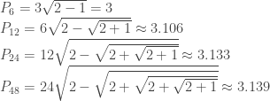
Liu Hui [刘徽] was a Chinese mathematician who lived in the Wei period. One of the things he was famous for was his method of calculating iteratively.

This approach to calculate (also used by Archimedes), is to calculate the area of a polygon inscribed in a circle. As the number of sides of the polygon increases, its area becomes closer and closer to the area of the circle.

Liu Hui found a simple formula to find the side length of an inscribed polygon of sides, if the side length of a polygon with sides is known:

Here is a temporary variable, and is the side length of an inscribed polygon with sides. Something like this:

We start with a hexagon. The radius of the circle is 1, the area . The side length of the hexagon is 1.

To calculate the next value, all we need to do is do an addition and a square root:

The area of a regular polygon is where is the number of sides, is the side length, and is the apothem. As the number of sides increases, the apothem becomes closer and closer to the radius, so here we’ll just let .

We then have the formula for the area of the polygon: , where is the area of a polygon with sides.

Let’s do a few here:

To save us some tedious work, here’s a Haskell program to do the calculations for us:

k 6 = 1
k n = sqrt $ 2 + k (n/2)
s n = sqrt $ 2 - k n
p n = (n/2) * s n
main = mapM_ (putStrLn . (\n -> show (round n) ++ " " ++ show (p n))) $ iterate (*2) 6

Here’s part of the output:

6 3.0
12 3.1058285412302498
24 3.132628613281237
48 3.139350203046872
96 3.14103195089053
192 3.1414524722853443
384 3.141557607911622
768 3.141583892148936
1536 3.1415904632367617
3072 3.1415921060430483
6144 3.1415925165881546
12288 3.1415926186407894
24576 3.1415926453212157
49152 3.1415926453212157
98304 3.1415926453212157

This is about the maximum you could get without arbitrary precision decimals: the area of a polygon with 98304 sides. This gives us 3.14159265 which is 8 digits of .

With a big-decimal library, it would be possible to calculate to any precision.

Happy pi day!