
The Pearson and Spearman correlation coefficients measure how closely two variables are correlated. They’re useful as an evaluation metric in certain machine learning tasks, when you want the model to predict some kind of score, but the actual value of the score is arbitrary, and you only care that the model puts high-scoring items above low-scoring items.
An example of this is the STS-B task in the GLUE benchmark: the task is to rate pairs of sentences on how similar they are. The task is evaluated using Pearson and Spearman correlations against the human ground-truth. Now, if model A has Spearman correlation of 0.55 and model B has 0.51, how confident are you that model A is actually better?
Recently, the NLP research community has advocated for more significance testing (Dror et al., 2018): report a p-value when comparing two models, to distinguish between true improvements and fluctuations due to random chance. However, hypothesis testing is rarely done for Pearson and Spearman metrics — it’s not mentioned in the hitchhiker’s guide linked above, and not supported by the standard ML libraries in Python and R. In this post, I describe how to do significance testing for a difference in Pearson / Spearman correlations, and give some references to the statistics literature.
Definitions and properties
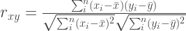
The Pearson correlation coefficient is defined by:
The Spearman rank-order correlation is defined as the Pearson correlation between the ranks of the two variables, and measures the relative order between them. Both correlation coefficients range between -1 and 1.
Pearson’s correlation is simpler, has nicer statistical properties, and is default option in most software packages. However, de Winter et al. (2016) argues that Spearman’s correlation works better with non-normal data and is more robust to outliers, so is generally preferred over Pearson’s correlation.
Significance testing
Suppose we have the predictions of model A and model B, and we wish to compute a p-value for whether their Pearson / Spearman correlation coefficients are different. Start by computing the correlation coefficients for both models against the ground truth.
Then, apply the Fisher transformation to each correlation coefficient:
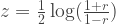
This transforms r which is between -1 and 1 into z, which ranges the whole real number line. It turns out that z is approximately normal, with nearly constant variance that only depends on N (the number of data points) and not on r.
For Pearson correlation, the standard deviation of the estimator 

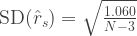
For Spearman rank-order correlation, the standard deviation of the estimator 
Now, we can compute the p-value because the difference of the two z values follows a normal distribution with known variance.
R implementation
The following R function computes a p-value for the two-tailed hypothesis test, given a ground truth vector and two model output vectors:
cor_significance_test <- function(truth, x1, x2, method="pearson") {
  n <- length(truth)
  cor1 <- cor(truth, x1, method=method)
  cor2 <- cor(truth, x2, method=method)
  fisher1 <- 0.5*log((1+cor1)/(1-cor1))
  fisher2 <- 0.5*log((1+cor2)/(1-cor2))
  if(method == "pearson") {
    expected_sd <- sqrt(1/(n-3))
  }
  else if(method == "spearman") {
    expected_sd <- sqrt(1.060/(n-3))
  }
  2*(1-pnorm(abs(fisher1-fisher2), sd=expected_sd))
}
Naturally, the one-tailed p-value is half of the two-sided one.
For details of other similar computations involving Pearson and Spearman correlations (eg: confidence intervals, unpaired hypothesis tests), I recommend the Handbook of Parametric and Nonparametric Statistical Procedures (Sheskin, 2000).
Caveats and limitations
The formula for the Pearson correlation is solid and very accurate. For Spearman, the constant 1.060 has no theoretical backing and was rather derived experimentally by Fieller et al. (1957), by running simulations using variables from a bivariate normal distribution. Fieller claimed that the approximation was accurate for correlations between -0.8 and 0.8. Borkowf (2002) warns that this approximation may be off if the distribution is far from a bivariate normal.
The procedure here for Spearman correlation may not be appropriate if the correlation coefficient is very high (above 0.8) or if the data is not approximately normal. In that case, you might want to try permutation tests or bootstrapping methods — refer to Bishara and Hittner (2012) for a detailed discussion.
References
- Dror, Rotem, et al. “The hitchhiker’s guide to testing statistical significance in natural language processing.” Proceedings of the 56th Annual Meeting of the Association for Computational Linguistics (Volume 1: Long Papers). Vol. 1. 2018.
- de Winter, Joost CF, Samuel D. Gosling, and Jeff Potter. “Comparing the Pearson and Spearman correlation coefficients across distributions and sample sizes: A tutorial using simulations and empirical data.” Psychological methods 21.3 (2016): 273.
- Sheskin, David J. “Parametric and nonparametric statistical procedures.” Chapman & Hall/CRC: Boca Raton, FL (2000).
- Fieller, Edgar C., Herman O. Hartley, and Egon S. Pearson. “Tests for rank correlation coefficients. I.” Biometrika 44.3/4 (1957): 470-481.
- Borkowf, Craig B. “Computing the nonnull asymptotic variance and the asymptotic relative efficiency of Spearman’s rank correlation.” Computational statistics & data analysis 39.3 (2002): 271-286.
- Bishara, Anthony J., and James B. Hittner. “Testing the significance of a correlation with nonnormal data: comparison of Pearson, Spearman, transformation, and resampling approaches.” Psychological methods 17.3 (2012): 399.
